Yu Gong , Yifei Wei , F. Richard Yu and Zhu Han
Slicing-Based Resource Optimization in Multi-Access Edge Network Using Ensemble Learning Aided DDPG Algorithm
Abstract: Recently, the technological development in edge computing and content caching can provide high-quality services for users in the wireless communication networks. As a promising technology, multi-access edge computing (MEC) can offload tasks to the nearby edge servers, which alleviates the pressure of users. However, various services and dynamic wireless channel conditions make effective resource allocation challenging. In addition, network slicing can create a logical virtual network and allocate resources flexibly among multiple tenants. In this paper, we construct an integrated architecture of communication, computing and caching to solve the joint optimization problem of task scheduling and resource allocation. In order to coordinate network functions and dynamically allocate limited resources, this paper adopts an improved deep reinforcement learning (DRL) method, which fully jointly considers the diversity of user request services and the dynamic wireless channel conditions to obtain the mobile virtual network operator (MVNO) maximal profit function. Considering the slow convergence speed of the DRL algorithm, this paper combines DRL and ensemble learning. The simulation result shows that the resource allocation scheme inspired by DRL is significantly better than the other compared strategies. The output of the result of DRL algorithm combined with ensemble learning is faster and more cost-effective.
Keywords: Content caching , deep reinforcement learning , ensemble learning , multi-access edge computing , network slicing
I. INTRODUCTION
IN recent years, smart devices and mobile users of wireless communication have been exponentially growing. The continuous development of mobile networks, wireless technology and the Internet of things (IoTs) have brought us a variety of powerful multimedia services and mobile applications. The fifth generation (5G) network provides a completely new vision of mobile networks, and contributes to meeting the different demands of various businesses. Network slicing refers to the flexible allocation of network resources. It is devoted to dividing multiple logical subnets with different characteristics according to requirements, and these subnets are isolated from each other [1]. Each end-to-end network slice that composed of the access network, transmission network, and core network sub-slices is managed uniformly through the slice management system. The technology of soft defined network (SDN) and network functions virtualization (NFV) [2], which are the basis of network slicing will lead the digital transformation of network infrastructure in the communication industry. In core networks or traditional cellular networks, entire systems are designed to support numerous types of services. However, a virtual wireless network composed with mobile virtual network operators (MVNO) is dedicated to one type of services (e.g., video transcoding and map downloading), which will give a better user experience. MVNO mainly focuses on abstracting and virtualizing the physical resources of the infrastructure provider (InP) into multiple network slices to satisfy the quality of service (QoS) of the network slice provider (SP) [3]. The role of MVNO, InP, and SP can be summarized as follows: 1) MVNO leases resources such as physical resources and backhaul bandwidth from InPs, generates virtual resources into different slices according to different users’ requests, and performs operations leases virtual resources to SPs. 2) InP that owned the radio resources of the physical networks (such as backhaul and spectrum) can operate the physical network infrastructure. 3) SP leases virtual resources to users for different services and various QoS requirements.
With the vigorous development of wireless communication networks and beyond, multi-service network supports a variety of application scenarios of diverse service requirements, and consequently generate a huge amount of contents and data [4]. These attractive services and applications heavily depend on low-latency transmission and high-speed data rates. However, the long distance between the users and the cloud server as well as the limited capacity of the backhaul link are significant challenges for satisfying the low-latency need of wireless communication networks and massive content delivery [5]. Therefore, with the continuous expansion of the number of users and the diversification of equipment application requirements, MVNO urgently needs to design systems that consist of QoS and quality of experience (QoE) to provide users with satisfaction services.
Multi-access edge computing (MEC) that deployed edge servers with certain computing resources and caching resources in small base stations (SBSs) is a promising paradigm. This technique can make full use of the network resources and satisfy the QoS of users [6]. It is placed part of the communication, computing and caching resources at the SBS equipped with the MEC server [7]. Consequently when the user requests resources, the MEC server can perform the corresponding tasks in a distributed manner, which will save backhaul bandwidth. The edge server in SBSs is lightweight and has limited resources, which compared with the central base station (BS). Therefore, it is urgent to find feasible resource allocation schemes for the computing and caching tasks requested by users. In addition, 5G technology guarantees the QoE of users and the QoS of network, but it is still a challenge to find the optimal scheme to allocate channel resources and bandwidth in a dynamic environment [8].
To overcome the challenge, as a crucial branch of artificial intelligence field, deep reinforcement learning (DRL) has the ability to recognize dynamic environments and has broad application prospects in solving resource allocation problems. It is different from convex optimization [9] and game theory [10] (assuming that the conditions of dynamic environment are fully already known) to solve the problems of resource allocation. The DRL method can widely solve the problem of complex resource allocation in the network slicing timevarying network. Some studies have applied DRL methods to manage resources, such as Deep-Q-Network (DQN) which is an effective approach to jointly schedule the resources for users [11]. DQN is suitable for solving discrete action space problems. However, the action space in our work is continuous. Therefore, this paper adopts the deep deterministic policy gradient (DDPG) [12] method that combines the actorcritic architecture with deep neural network (DNN) to solve the resource allocation problem.
Based on the method of DRL, an agent can choose the optimal action in a fairly complex environment. However, deep reinforcement learning has few practical applications in industry, mainly due to the very expensive computational cost and the black-box nature of its model [13]. In [13], it is proposed that the solution obtained through deep reinforcement learning can be converted into a gradient boosting decision tree (GBDT) model by the distillation methods that are widely used in the imaging field. GBDT is a member of the family of boosting algorithms and it is also a sub-branch of ensemble learning [14], which is the process of combining multiple single models to form a better model. It can show the importance of input parameters as well as calculate the output more economically and faster in the GBDT model, compared with the DRL method. Therefore, considering the limitations of DRL and the high computational cost, this paper proposes the ensemble learning aided DRL algorithm.
This paper studies the joint problem of edge computing and content caching, and builds a comprehensive architecture that is integrated by communication, computing and caching resources. Furthermore, we put forward a problem that jointly optimizes the task scheduling and resource allocation. We weight the QoS of users and the benefit of operator with the purpose of maximizing the profit of operator. In order to coordinate network functions, dynamically allocate limited resources, and fully consider the diversity of user service requests and the time-varying state of the channel, we use an improved DRL method to obtain the MVNO maximized profit function. The main contributions of this article can be summarized as follows:
· We propose a model of MEC and caching, which jointly considers the resources of communication, computing, and caching. In this model, the SBS can perform computation tasks and deliver caching content, and the BS equipped with a controller will complete task scheduling and resource allocation.
· We design a novel profit function to measure the performance of MVNO, which takes the revenue of MVNO and the QoE of users into account. Furthermore, we propose a joint optimization problem that is used to maximize the revenue of MVNO by allocating tasks and resources in wireless communication network.
· We adopt a solution of the edge computing and caching based DDPG algorithm. This solution considers the diversity of services requested by users and dynamic communication conditions between MEC servers and users to jointly optimize task scheduling and resource allocation in a continuous action space.
· We use the data set generated by the DDPG algorithm to train the GBDT model. After training, the GBDT model can completely imitate the behavior of the DDPG agent and the output of results is faster and more cost-effective.
The remainder of this paper can be organized as follows. We review the related works in Section II. The system model is presented in Section III. We describe the edge computing and caching scheduling as an optimization problem in Section IV. And the GBDT-based DDPG algorithm designed to solve the proposed optimization problem is shown in Section V. Simulation results are proposed in Section VI and the conclusion is provided in Section VII.
II. RELATED WORK
A. Research on Slicing-Based Resource Optimization
In academia and industry, there are a large number of researchers have great interest in studying the applications of network slicing technology and resource optimization for MEC systems. Jointly considering the tasks of computation offloading and power allocation, some studies have proposed a new framework that combined the MEC system with network slicing. The authors in [15] formulated the problem as a mixed integer nonlinear programming problem that is solved by convex optimization method. The authors in [9] used the Lyapunov optimization technology to optimize the task of computing offloading and power allocation, which can maximize the average income of operators. There are also some studies that solved the problem of computing and communication resource allocation among multiple tenants. The problem can be solved by various algorithms such as the upper-tier first with the latency-bounded over-provisioning prevention (UFLOP) algorithm proposed in [16], the convex optimization used in [17], and the computational load distribution algorithm adopt in [18]. In addition, the authors in [19] jointly considered communication and computing resources and used the DQN algorithm to maximize the utility of MVNO.
The diversification of 5G network scenarios requires effective allocation of multi-dimensional resources such as communication, computation, and cache in terms of delay, bandwidth, and connectivity according to different service requirements. Therefore, there are a large number of researches have focused on the resource allocation in network slicing. The works in [20] and [21] were jointly optimizing caching resources and communication resources. The studies in [22] and [23] were jointly optimizing computing resources and communication resources, which have adopted the algorithm of Q-Learning and convex optimization respectively. In fact, the integration and collaboration between communication, computing and caching resources are the main research direction in the future. However, most of existing research focus on optimization of communication and computing, caching and communication or computing and power allocation. This paper describes a joint optimization problem of these three resources allocation, and proposes the DDPG algorithm to maximize the profit of MVNO while ensuring the QoS of users in our wireless communication system.
B. Research on GBDT
On the other hand, tree models and neural networks are like two sides of a coin. In certain cases, the performance of the tree model is even better than the performance of the neural network. The authors evaluated the model with the robot verification system as the opponent in [24], which proved that the model combined GBDT and neural network have the best win-rate compared with GBDT-only and neural networkonly. GBDT is one of the best algorithms for fitting the true distribution among traditional machine learning algorithms. The authors in [25] proposed that the future travel time can be predicted based on the information of historical taxi trajectory. The authors in [26] used the GBDT model to construct the multi-dimensional basic features with original data to further improve the prediction accuracy. The risk prediction model proposed in [27] is based on the combination of GBDT and logistic, which is used to solve the problem of bad debts of telecom operators caused by fraudulent account overdraft fees of some mobile communication users.
In fact, as far as we know, few works apply the GBDT method to solve the problems of resource allocation, or even other problems of regression in the communication systems. The authors in [28] used the DQN algorithm to effectively solve the problem of resource allocation in the high-dimensional state. In addition, in order to solve the problem that DQN is difficult to obtain rewards under lowdelay conditions, a tree-based gradient-enhanced decision tree is used to approximate the second order cone programming (SOCP) solution. However, in our system model, the problem that needs to be optimized is almost impossible to approximate the optimal solution through GBDT. The authors in [13] proposed a method that combines GBDT and deep reinforcement learning. It used XGBoost (usually used as a GBDT model) to build a model, and proved that the GBDT model has more than five-fold the speed advantage while performing on par with deep reinforcement learning agents. We learn from this idea and apply this method to solve the problem of resource allocation in our system. The goal is maximizing the benefits of MVNO.
III. SYSTEM MODEL
A. Network Model
As shown in Fig. 1, we consider that the network consists of one BS deployed with the controller and several SBSs equipped with MEC servers for serving multiple users. Users can request multiple types of services, and different services can be treated as different slices of the network. Furthermore, the coverage areas of SBSs are overlapped, so as to ensure that each user with a service request is associated with an SBS. We assume that each user with a service request can be associated with only one SBS in the same time slot.
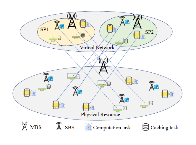
Let 𝒱 = {1, 2, · · ·, V } represent the set of users and 𝒰 = {1, 2, · · ·,U} represent the set of SBSs. The services requested by users can be divided into computation offloading and content delivery. We assume that the request packets have flags, which can distinguish the service types of different services [29].
Let 𝒩 = {1, 2, · · ·,N} represent the set of users that request computation offloading and ℳ = {1, 2, · · ·,M} represent the set of users that request content delivery. We assume that the user can only admit one service request at the same time, so that the number of users requested service can be defined as N + M = V . In addition, 𝒮 = {1, 2, · · ·, S} represents the set of SPs. For each SP s, allocated with user v can be regarded as a set that is defined as [TeX:] $$V_s$$, where [TeX:] $$V=\cup_s V_s$$ and [TeX:] $$V_s \cap V_{s^{\prime}}=\emptyset, \forall s^{\prime} \neq s .$$
Table I list the main parameters in this paper.
TABLE I
| Parameters | Definition |
|---|---|
| 𝒱 | The set of users |
| 𝒰 | The set of SBSs |
| ℳ | The set of users requested computation offloading task |
| 𝒩 | The set of users requested content delivery task |
| 𝒮 | The set of SPs |
| [TeX:] $$v_{s_k}$$ | The user v omitted request service SP s |
| [TeX:] $$a_{v_{s_k}, u}$$ | The task established indicator between user [TeX:] $$v_{s_k}$$ and SBS u |
| [TeX:] $$b_{v_{s_k}, u}$$ | The subchannels allocated to user [TeX:] $$v_{s_k}$$ form SBS u |
| [TeX:] $$\Gamma_{v_{s_k}, u}$$ | The average SINR between user [TeX:] $$v_{s_k}$$ and SBS u |
| [TeX:] $$r_{v_{s_k}, u}$$ | The data transmission rate between user [TeX:] $$v_{s_k}$$and SBS u |
| [TeX:] $$\sigma^2$$ | The additive white Gaussian noise |
| [TeX:] $$P_{v_{s_k}}$$ | The transmission power of user [TeX:] $$v_{s_k}$$ |
| [TeX:] $$h_{v_{s_k}, u}$$ | The average channel gains between user [TeX:] $$v_{s_k}$$ and SBS u |
| [TeX:] $$B_u$$ | The spectrum bandwidth which allocated to SBS u |
| [TeX:] $$D_{v_{s_k}}$$ | The input-data size of the computation task requested by user[TeX:] $$v_{s_k}$$ |
| [TeX:] $$X_{v_{s_k}}$$ | The computing ability of the computation task requested by user[TeX:] $$v_{s_k}$$ |
| [TeX:] $$f_{v_{s_k}, u}$$ | The computational capability of SBS u assigned to user [TeX:] $$v_{s_k}$$ |
| [TeX:] $$e_u$$ | The energy consumption at SBS u per CPU cycles |
| [TeX:] $$R_{v_{s_k}, u}$$ | The computation rate between user [TeX:] $$v_{s_k}$$ and SBS u |
| [TeX:] $$E_{v_{s_k}, u}$$ | The total energy consumption between user [TeX:] $$v_{s_k}$$ and SBS u during the computational task |
| [TeX:] $$F_u$$ | The computing capability allocated to SBS u |
| [TeX:] $$c_{v_{s_k}}$$ | The caching content capacity of user [TeX:] $$v_{s_k}$$ |
| [TeX:] $$g_{v_{s_k}, u}$$ | The expected saved backhaul bandwidth between user [TeX:] $$v_{s_k}$$ and SBS u by caching content |
| [TeX:] $$p_f$$ | The probability of the content F |
| [TeX:] $$T_{v_{s_k}, u}$$ | The time durations of user [TeX:] $$v_{s_k}$$ to download the required content from SBS u via the backhaul |
| [TeX:] $$C_u$$ | The caching space allocated to SBS u |
| [TeX:] $$\lambda_{v_{s_k}, u}$$ | The virtual network access fee of users [TeX:] $$v_{s_k}$$ charged by MVNO, is [TeX:] $$\lambda_{v_{s_k}, u}$$ per bps |
| [TeX:] $$\mu_{v_{s_k}, u}$$ | The spectrum usage cost at SBS u, paid by MVNO, is [TeX:] $$\mu_{v_{s_k}, u}$$ per Hz |
| [TeX:] $$\phi_{v_{s_k}, u}$$ | The fee of computation offloading of user [TeX:] $$v_{s_k}$$, charged by MVNO, is [TeX:] $$\phi_{v_{s_k}, u}$$ per bps |
| [TeX:] $$\Phi_{v_{s_k}, u}$$ | The price of computation energy at SBS u, paid by MVNO, is [TeX:] $$\Phi_{v_{s_k}, u}$$ |
| [TeX:] $$\psi_{v_{s_k}, u}$$ | The fee of content delivery of user [TeX:] $$v_{s_k}$$, charged by MVNO, is [TeX:] $$\psi_{v_{s_k}, u}$$ per bps |
| [TeX:] $$\Psi_{v_{s_k}, u}$$ | The price of the gains of the expected saved backhaul bandwidth at SBS u, paid by MVNO, is [TeX:] $$\Psi_{v_{s_k}, u}$$ per byte |
| γ | The TD errors |
| [TeX:] $$\omega_t$$ | The discount factor |
| [TeX:] $$\theta_t$$ | The parameter of value function |
| [TeX:] $$\alpha_\omega, \alpha_\theta$$ | The parameter of policy |
| τ | The learning rate of critic and actor |
| β, λ | The soft update parameter |
B. Communication Model
There are 𝓀 users omit request service SP s, so the set of users that omitted service s can be represented as [TeX:] $$V_s=\left\{v_{s_1}, v_{s_2}, \cdots, v_{s_K}\right\}$$. Regard [TeX:] $$a_{v_{v_{s_k}}, u}$$ as the task established indicator, where [TeX:] $$a_{v_{s_k}, u}=1$$ denotes that user 𝓋 requests the SP s and associates with SBS u; otherwise [TeX:] $$a_{v_{s_k}, u}=0$$. Specially, each user can be associated with only one SBS, which is defined as [TeX:] $$\Sigma_{u \in U} a_{v_{s_k}, u}=1, \forall s \in S, \forall v_{s_k} \in V_s$$.
The total spectrum bandwidth of all SBSs can be defined as B, which is [TeX:] $$B=\sum_u B_u$$. [TeX:] $$B_u$$ represents the spectrum bandwidth allocated to SBS u. Practically, the bandwidth of SBS [TeX:] $$B_u$$ Hz can be divided into [TeX:] $$B_u / \mathcal{B}$$ subchannels, and the subchannels allocated to user [TeX:] $$v_s$$ is [TeX:] $$b_{v_{s_k}, u} \in\left\{1,2, \cdots, B_u / \mathcal{B}\right\}$$. Therefore [TeX:] $$B_u$$ can be denoted as
(1)
[TeX:] $$\Sigma_{s \in S} \Sigma_{v_{s_k} \in V_s} a_{v_{s_k}, u} b_{v_{s_k}, u} \mathcal{B} \leq B_u, \forall u \in \mathcal{U}$$where [TeX:] $$b_{v_{s_k}, u} \mathcal{B}$$ is the allocated bandwidth from SBS u to user [TeX:] $$v_{s_k}$$.
We assume that SBSs belong to different InPs, so that the licensed spectrum of each InP is orthogonal. Therefore, there are no interference between different SBSs. However, there exists interference between users that belonged to the same SP and connected to the same SBS. The average signalinterference- noise ratio (SINR) between user [TeX:] $$v_s$$ and SBS u can be defined as
(2)
[TeX:] $$\Gamma_{v_{s_k}, u}=\frac{P_{v_{s_k}} h_{v_{s_k}, u}}{\sum_{i \in \mathcal{K}, i \neq k} P_{v_{s_i}} h_{v_{s_i}, u}+\sigma^2},$$where [TeX:] $$P_{v_{s_k}}$$ and [TeX:] $$P_{v_{s_i}}$$ represent the transmission power of user [TeX:] $$v_{s_k}$$ and user [TeX:] $$v_{s_i}$$, respectively. [TeX:] $$h_{v_{s_k}, u}$$ and [TeX:] $$h_{v_{s_i}, u}$$ are average channel gains. [TeX:] $$\sigma^2$$ is additive white Gaussian noise (AWGN).
Furthermore, the rate of data transmission between SBS u and user [TeX:] $$v_{s_k}$$ can be calculated by the Shannon theory, i.e.,
(3)
[TeX:] $$r_{v_{s_k}, u}=b_{v_{s_k}, u} \mathcal{B} \log _2\left(1+\Gamma_{v_{s_k}, u}\right) .$$The quasi-static assumption have be used in this paper, which means that the state of the environment remains unchanged within the time slot t.
C. Computing Model
The computing task of user [TeX:] $$v_{s_k}$$ can be described as [TeX:] $$J_{v_{s_k}}=\left\{D_{v_{s_k}}, X_{v_{s_k}}\right\}$$, where [TeX:] $$D_{v_{s_k}}$$ represents the input-data size (bits) and [TeX:] $$X_{v_{s_k}}$$ represents the computing ability (i.e., the total number of CPU cycles to compute the task) of the computation task requested by user [TeX:] $$v_{s_k}$$. In addition, [TeX:] $$f_{v_{s_k}, u}$$ is the computational capability of SBS u assigned to user [TeX:] $$v_{s_k}$$ (i.e., the total number of CPU cycles per second) [30].
Therefore, the total execution time of computational task [TeX:] $$J_{v_{s_k}}$$ at SBS u can be calculate by [TeX:] $$t_{v_{s_k}, u}=X_{v_{s_k}} / f_{v_{s_k}, u}$$. The computation rate which is quantized by the amounts of bits per second can be easily obtained by
(4)
[TeX:] $$R_{v_{s_k}, u}=\frac{D_{v_{s_k}}}{t_{v_{s_k}, u}}=\frac{D_{v_{s_k}} f_{v_{s_k}, u}}{X_{v_{s_k}}}.$$The total consumption of energy during computational task [TeX:] $$J_{v_{s_k}}$$ can be represented as
where [TeX:] $$e_u$$ represents the energy consumption at SBS u per CPU cycles.
Moreover, the computing ability is limited at each SBS, i.e.,
(6)
[TeX:] $$\Sigma_{s \in \mathcal{S}} \Sigma_{v_{s_k} \in V_s} a_{v_{s_k}, u} f_{v_{s_k}, u} \leq F_u, \forall u \in \mathcal{U},$$where [TeX:] $$F_u$$ is the computing capability allocated to SBS u. Practically, the total computing capability of all SBSs can be defined as F, which is [TeX:] $$F=\sum_u F_u$$.
D. Caching Model
The caching task of user [TeX:] $$v_{s_k}$$ can be described as [TeX:] $$c_{v_{s_k}}$$. In this paper, it is assumed that the storage of SBSs is limited which can store only F type popular contents. Therefore, the set of cached content can be regard as library, i.e., ℱ = {1, 2, · · ·, F} [29]. Without loss of generality, the number of contents is always F.
contents is always F. The probability of the content F requested by user obeys the Zipf distribution [31], which is modeled as
where parameter ι indicates the popularity of content, and it is always a positive value. In our caching model, the popularity of content can be directly calculated from the formulation if the content caching task omitted by the user has been known.
In addition, [TeX:] $$T_{v_{s_k}, u}$$ is the time to download the required content through the backhaul. Therefore, the expected backhaul bandwidth savings obtained by caching content can be expressed by
where [TeX:] $$p_{v_{s_k}, u}$$ can be calculated directly by (7).
In general, the content cached with a lower degree of popularity will be cost higher price. In other words, some of this content may not be cached in the SBS because it doesn’t make any sense. Actually, many scholars have studied the pricing of caching systems [32]. In our work, we consider a caching strategy which the prices of different contents are already known.
Moreover, the caching space is limited at each SBS, i.e.,
(9)
[TeX:] $$\Sigma_{s \in S} \Sigma_{v_{s_k} \in V_s} a_{v_{s_k}, u} c_{v_{s_k}, u} \leq C_u, \forall u \in \mathcal{U},$$where [TeX:] $$C_u$$ is the caching space allocated to SBS u. Practically, the total caching space of all SBSs can be defined as C, which is [TeX:] $$C=\sum_u C_u$$.
IV. PROBLEM FORMULATION
The profit function has been defined in this section and it is used to calculate the total profits of MVNO. In order to maximize the profit function, this paper designs the optimization objective that jointly considers the resource allocation and task assignments to maximize the system performance such as the utility of MVNO.
A. Profit Function
Particularly, the resource consumption that consists of computing, caching and communication is considered in this paper. The virtual network access fee charged by MVNO from users [TeX:] $$v_{s_k}$$ is [TeX:] $$\lambda_{v_{s_k}, u}$$ per bps. After paying the fees to MVNO, the user has the right to access the physical resource and complete the task. On the other hand, MVNO also pays the usage of spectrum which is [TeX:] $$\mu_{v_{s_k}, u}$$ per Hz for InPs. If the task user requested is computation offloading, MVNO may charge the fee of [TeX:] $$\phi_{v_{s_k}, u}$$ per bps from users [TeX:] $$v_{s_k}$$. Meanwhile, MVNO will pay the computation energy cost that can be defined as [TeX:] $$\Phi_{v_{s_k}, u}$$ per J for SBS u. If the task is caching delivery, MVNO may charge the fee of [TeX:] $$\psi_{v_{s_k}, u}$$ per bps. Meanwhile, MVNO will pay the price of caching at the SBS, which is defined as [TeX:] $$\Psi_{v_{s_k}, u}$$ per byte for SBS u.
So the profit function between user [TeX:] $$v_{s_k}$$ and SBS u for the potential transmission can be defined as
The total profits of the MVNO can be divided as three components, i.e., communication, computation, and caching proceeds.
1) Communication proceeds: The first term of the above profit function is the communication revenue. [TeX:] $$\lambda_{v_{s_k}, u} r_{v_{s_k}, u}$$ represents the revenue which the user [TeX:] $$v_{s_k}$$ pay for MVNO to access the virtual networks, and [TeX:] $$\mu_{v_{s_k}, u} b_{v_{s_k}, u} \mathcal{B}$$ denotes the bandwidth spending of MVNO pay for InP.
2) Computing proceeds: The second term of the above profit function is the computation revenue. [TeX:] $$\phi_{v_{s_k}, u} R_{v_{s_k}, u}$$ represents the revenue which the user [TeX:] $$v_{s_k}$$ pay for MVNO to execute the computation task, and [TeX:] $$\Phi_{v_{s_k}, u} E_{v_{s_k}, u}$$ denotes the energy consumption spending of MVNO pay for InP.
3) Caching proceeds: The last term of the above profit function is the caching revenue. [TeX:] $$\psi_{v_{s_k}, u} g_{v_{s_k}, u}$$ represents the revenue which the user [TeX:] $$v_{s_k}$$ pay for MVNO to execute the caching task, and [TeX:] $$\Psi_{v_{s_k}, u} c_{v_{s_k}, u}$$ denotes the spending of MVNO caching content [TeX:] $$c_{v_{s_k}, u}$$.
B. Optimization Objective
Mathematically speaking, the total profit of MVNO that renting the three resources can be maximized, by continuously optimizing the task assignment and resource allocation between InP and NSP. Specifically, the communication proceeds [TeX:] $$\left(\lambda_{v_{s_k}, u} r_{v_{s_k}, u}-\mu_{v_{s_k}, u} b_{v_{s_k}, u} \mathcal{B}\right)$$, computing proceeds [TeX:] $$\left(\phi_{v_{s_k}, u} R_{v_{s_k}, u}-\Phi_{v_{s_k}, u} E_{v_{s_k}, u}\right),$$ and caching proceeds [TeX:] $$\left(\psi_{v_{s_k}, u} g_{v_{s_k}, u}-\Psi_{v_{s_k}, u} c_{v_{s_k}, u}\right)$$ of MVNO are influenced by the allocation of communication, computing and caching resources. Therefore, the optimization objective of this paper is to maximize the total profits of MVNO, which is calculated by
(10)
[TeX:] $$O P: \max _{\left\{b_{v_{s_k}, u}, f_{v_{s_k}, u}, c_{v_{s_k}, u}\right\}} \sum_{s \in \mathcal{S}} \sum_{v_{s_k} \in V_s} \sum_{u \in \mathcal{U}} U_{v_{s_k}, u} .$$
Constraint C1 represents that user [TeX:] $$v_{s_k}$$ can only associate with one SBS u. Furthermore, C2 reflects that the allocated bandwidth from SBS u to all users associated with it cannot exceed the spectrum resource of SBS u. Constraints C3 and C5 ensure the requirements of each user [TeX:] $$v_{s_k}$$ which consist of communication rate [TeX:] $$r_{v_{s_k}}^{\mathrm{cm}}$$ and computing rate [TeX:] $$R_{v_{s_k}}^{\mathrm{cp}},$$ respectively. According to C4 and C6, we define that the computing ability [TeX:] $$F_u$$ and and caching space [TeX:] $$C_u$$ of each SBS u are limited.
V. PROPOSED SOLUTION WITH GBDT-BASED DDPG ALGORITHM
Game theory [33] and convex optimization [6] are two common methods which used to solve the problems of edge computing and content caching. However, such methods need to know key factors (e.g., content popularity, dynamic wireless channel condition), which are unavailable and time-varying in reality. It is a challenge to guarantee reliable and efficient data transmissions caused by the diversity of user service requests. Compared with the above methods, DRL can solve the problem of high-dimensional and time-varying characteristics, and can utilize deep neural network to allocate resources efficiently [34].
In order to maximize the total profits of MVNO and solve the optimization problem that jointly considers the task assignment and resource allocation, we formulate it as the stochastic sequential decision problem (SDP). The Markov decision process (MDP) framework has been used to solve SDP problem. Reinforcement Learning can be described as a MDP to find the optimal strategy. Therefore, the above optimization objective will be described as a reinforcement learning problem.
A. Definition of Reinforcement Learning
The controller deployed at the BS can be seen as the agent, which can interact with environment (i.e., collect all information of the system state) and obtain a reward after executing action (i.e., make decisions for all requests). The target of controller is to maximize the reward not as an immediate return but a long-term cumulative one. The process to explore the optimal strategy can be regarded as: The agent observes the state information [TeX:] $$s_t \in \mathcal{S}$$ at time slot t and then selects the action [TeX:] $$a_t \in \mathcal{A}$$, based on the strategy [TeX:] $$\pi(a \mid s)$$ (indicates the probability of choosing action under the state); after taking action [TeX:] $$a_t$$, the agent receives the immediate return. Generally, the target of MDP is exploring a strategy [TeX:] $$\pi(a \mid s)$$ to maximize the value function, which is usually expressed by the expected discounted cumulative return calculated by the Bellman equation [35].
Three key elements which consist of space of state, space of action and reward in this paper are introduced as follows.
1) Space of state: In our system, the state space concludes two components that are the available resources of each SBS [TeX:] $$u(u \in \mathcal{U})$$ equipped with MEC servers and the status of each user [TeX:] $$v(v \in \mathcal{V})$$. At time slot t the state space can be denoted as
[TeX:] $$F_u, B_u$$, and [TeX:] $$C_u$$ represent the available resources (e.g., computing, bandwidth, and caching) of each SBS u [TeX:] $$u(u \in \mathcal{U})$$ equipped with MEC servers. In addition, the status of each user [TeX:] $$\Omega_v$$ includes the average SINR between the user and SBS, the input-data size (bits) of the computation task, the computing ability (the total number of CPU cycles to complete the task), the capacity of caching, the content popularity and the requested service type of the user.
2) Space of action: The agent in our system decides how many network resources will be allocated to the users. Specifically, after receiving various requests from users, the system will schedule the resources from the SBS that equipped with MEC servers. The target is completing the computing offloading or content delivery task. At time slot t, the action space can be denoted as
[TeX:] $$b_{v_{s_k}, u}, f_{v_{s_k}, u}$$, and [TeX:] $$c_{v_{s_k}, u}$$ represents the amount of bandwidth, computing resources, and caching resources that the SBS equipped with MEC servers u allocated to user [TeX:] $$v_{s_k}$$, respectively.
3) Reward: After taking action [TeX:] $$a_t$$, the agent will receivethe agent will receive reward [TeX:] $$R_t$$. Particularly, the reward should be corresponding with the above optimization objective function. Thus, the reward can be defined as
(13)
[TeX:] $$R_t=\sum_{s \in \mathcal{S}} \sum_{v_{s_k} \in V_s} \sum_{u \in \mathcal{U}} U_{v_{s_k}, u}.$$B. Policy and Value Function
Almost all reinforcement learning algorithms involve evaluating state (or action) value functions to estimate the expected return for a given state (or action performed in the given state). In order to calculate the value of strategy π, the state value function defined by the expectation description can be represented by
(14)
[TeX:] $$v_\pi(s)=\mathbb{E}_\pi\left[\sum_{k=0}^{\infty} \gamma^k R_{t+k+1} \mid s_t=s\right],$$where [TeX:] $$\gamma \in[0,1]$$ denotes as the discount factor that is used to calculate the cumulative reward.
In the Markov decision process, the action value of action a under strategy π and state s is often evaluated, which is defined as an action value function and expressed as
(15)
[TeX:] $$q_\pi(s, a)=\mathbb{E}_\pi\left[\sum_{k=0}^{\infty} \gamma^k R_{t+k+1} \mid s_t=s, a_t=a\right].$$Value-based reinforcement learning algorithms basically learn value functions (including action and state value functions), and then select actions according to the obtained values. The goal of the agent is choosing the action that can maximize the cumulative reward. The generalized value function method includes two steps: Strategy evaluation and strategy improvement. When the value function is optimal, the optimal strategy at this time is greedy strategy. Greedy strategy refers to selecting the action corresponding to the maximum Q-value under state s. Another common strategy is ε − greedy, where the agent selects the action corresponding to the maximum action value function with ε probability.
In the value-based learning method, the value function is calculated iteratively. In the policy-based learning method, the strategy parameters are directly calculated iteratively until the cumulative return is the maximum. After that, the strategy corresponding to the parameters is the optimal strategy. The role of the value function is to learn the parameters of policy, not the choice of action. In the policy parameterization method, θ is used as the parameter factor of the policy. Then the probability that the policy function, in state s and select action a at time slot t, can be defined as
The optimal policy π* can be learned by the method of policy gradient [36]. Moreover, the actual output of the policy gradient method is the action probability distribution, so it is also called stochastic policy gradient (SPG). When the action is a high-dimensional vector, it is computationally intensive to sample action for the strategy generated randomly. The deterministic behavior strategies are directly generated by deterministic policy gradient (DPG) that is used to solve the calculation problem caused by frequent action sampling. After that, each step of the action will obtain a unique deterministic value through the policy function. It has been proved that deterministic policy gradient is a limit form of stochastic policy gradient through rigorous mathematical derivation in [37].
The deterministic strategy is denoted by [TeX:] $$\mu_\theta,$$, and the objective function is the accumulated return obtained by
Combined with the objective function, the gradient expression of the deterministic strategy gradient objective function can be obtained by
(18)
[TeX:] $$\begin{aligned} \nabla_\theta J\left(\mu_\theta\right) & =\left.\int_S \rho^\mu(s) \nabla_\theta \mu_\theta(s) \nabla_a Q^\mu(s, a)\right|_{a=\mu_\theta(s)} d s \\ & =\mathbb{E}_{s \sim \rho^\mu}\left[\left.\nabla_\theta \mu_\theta(s) \nabla_a Q^\mu(s, a)\right|_{a=\mu_\theta(s)}\right], \end{aligned}$$where [TeX:] $$\rho^\mu$$ is the discounted state visitation distribution of deterministic policy μ.
C. Deep Deterministic Policy Gradient Algorithm
The DDPG algorithm is combined the idea of DPG with actor-critic. The update rules of the three main parameters involved in the algorithm are as follows:
(19)
[TeX:] $$\delta_t=r_t+\gamma Q^\omega\left(s_{t+1}, \mu_\theta\left(s_{t+1}\right)\right)-Q^\omega\left(s_t, a_t\right),$$
(20)
[TeX:] $$\omega_{t+1}=\omega_t+\alpha_\omega \delta_t \nabla_\omega Q^\omega\left(s_t, a_t\right),$$
(21)
[TeX:] $$\theta_{t+1}=\theta_t+\left.\alpha_\theta \nabla_\theta \mu_\theta\left(s_t\right) \nabla_a Q^\omega\left(s_t, a_t\right)\right|_{a=\mu_\theta\left(s_t\right)},$$where [TeX:] $$\delta_t$$ denotes temporal-difference (TD) errors. [TeX:] $$\omega_{t+1}$$ and [TeX:] $$\theta_{t+1}$$ represent the parameter of value function and policy, respectively. [TeX:] $$\alpha_\omega$$ and [TeX:] $$\alpha_\theta$$ denotes the learning rate of critic and actor, respectively.
The method of value function approximation is used to update the parameters of [TeX:] $$\delta_t$$ and [TeX:] $$\omega_{t+1}$$, and the parameter of policy [TeX:] $$\theta_{t+1}$$ is updated by the deterministic strategy gradient method.
The DDPG algorithm is based on the actor-critic structure: the actor uses the deterministic policy gradient method to learn the optimal behavior strategy; the critic uses the Q-learning method to evaluate and optimize the action value function. The two functions are fitted by the convolutional neural network, and the samples need to be independently and identically distributed. However, the samples generated in reinforcement learning are collected sequentially and have the Markov characteristics. Additionally, it is important to learn in mini-batches, rather than the online manner [12]. In the DQN algorithm, the replay buffer is used to solve these problems. Inspired by the advantages of DQN, the DDPG algorithm applies experience relay and target network (Target-Q) to improve the stability of convergence.
1) Experience replay: The agent obtains the data tuple [TeX:] $$\left(s_t, a_t, r_t, s_{t+1}\right)$$ by interacting with the environment and stores it in the experience pool (replay buffer). When the actor and critic networks need to be updated, minibatch sampling is performed from the experience pool denoted as [TeX:] $$\left(s_t, a_t, r_t, s_{t+1}\right)$$. If the amount of data stored in the experience pool reaches a peak, the old data will be automatically discarded. DDPG is an off-policy algorithm, and so the replay buffer should be sufficiently large to achieve as far as possible that the samples selected during the update process are completely irrelevant.
2) Target network: There exists two target networks in DDPG, corresponding to the actor and critic. Different from the parameter update mode of the Target-Q network in DQN (the value network parameters are directly copied after a fixed interval), DDPG adopts a soft parameter update mode. Assuming that the parameter of the actor target network is [TeX:] $$\theta^{\mu^{\prime}}$$ and the parameter of the critic target network is [TeX:] $$\theta^{Q^{\prime}}$$. The parameter update rule in soft mode is:
where τ is the soft update parameter and the condition τ ≪ 1 improves the training stability.
This parameter update method is similar to supervised learning, which can greatly improve the stability of learning, but the problem is that the update speed is slow.
D. Gradient Boosting Decision Tree Algorithm
Gradient boosting machine (GBM) is a very commonly ensemble learning algorithm. It can be regarded as a gradient enhancement framework composed of various classifiers or regressors or regarded as a collection of basic estimators. The basic estimator such as naive Bayesian estimators, K-nearest neighbor and neural network can be fitted to GBM [28]. It is worth mentioning that the better the basic estimator, the higher the system performance.
There are many types of GBM, the most classical is GBDT that is based on decision trees. GBDT is an iterative decision tree algorithm that is very different from the traditional Adaboost algorithm. The authors in [38] proposed a scalable end-to-end tree boosting system which is called XGBoost. It is an improved GBDT algorithm. In particular, GBDT only uses the information of the first-order derivative in optimization, while the XGBoost algorithm uses the first-order and secondorder derivatives to perform a second-order Taylor expansion of the cost function. In addition, a regular term contained the number and the score function of each tree leaf nodes is added to the cost function and it can control the complexity of the model.
In our framework, we use the improved GBDT algorithm which is applied to regression tasks. Given a dataset of n samples. The dataset can be represented as
(24)
[TeX:] $$D=\left(x_i, y_i\right)\left(|D|=n, x_i \in F \cup B \cup C \cup \Omega, y_i \in \mathcal{R}\right),$$where [TeX:] $$x_i$$ expressed as the state space [TeX:] $$\left[F_1^i, F_2^i, \cdots, F_u^i ; B_1^i, B_2^i\right.,\left.\cdots, B_u^i ; C_1^i, C_2^i, \cdots, C_u^i ; \Omega_1^i, \Omega_2^i, \cdots, \Omega_v^i\right]$$ of our system model. [TeX:] $$y_i$$ represented as the solution according to the reward function.
The model of tree ensemble uses the K additive function to predict the output, which is expressed as
where ℱ represents the space of CART trees.
We need to minimize the regularized objective function to learn the function set of the model, i.e.,
where [TeX:] $$\hat{y}_i$$ represent the predicted value and [TeX:] $$y_i$$ is the true target value corresponding to the reward function. Here the first term of the differentiable convex function L predicts the loss of the model, which is used to measure the gap between the true profits and estimated profits of MVNO. The second term of the function is a regular penalty that limits the complexity of the model.
The penalty function can be calculated by
where where T represents the number of leaves and w denotes the weight owned by each leaf in the tree. There exists two typical hyper-parameters: β and λ.
Equation (25) is difficult to optimize, and we add [TeX:] $$f_t$$ minimize the objective function, i.e.,
(28)
[TeX:] $$L^{(t)}=\sum_{i=1}^n l\left(y_i, \hat{y}_i^{(t-1)}+f_t\left(x_i\right)\right)+\Omega\left(f_t\right).$$We take the second-order approximation to quickly optimize the objective in the general setting, i.e.,
(29)
[TeX:] $$L^{(t)} \cong \sum_{i=1}^n\left[l\left(y_i, \hat{y}_i^{(t-1)}\right)+g_i f_t\left(x_i\right)+\frac{1}{2} h_i f_t^2\left(x_i\right)\right]+\Omega\left(f_t\right),$$where [TeX:] $$g_i$$ is a gradient of the loss function and [TeX:] $$h_i$$ is the second step of the loss function.
The scoring function used to measure the quality of a tree structure is omitted in this article, and the reader can check the reference for the specific derivation [27].
The final prediction result of GBDT is a linear combination of K regression trees, represented as
where [TeX:] $$f_0(x)$$ is the initial predicted value, and [TeX:] $$\phi_k(x)$$ and [TeX:] $$\theta_k$$, respectively, represent the base estimator and its corresponding weight.
E. Gradient Boosting Decision Tree Based Deep Deterministic Policy Gradient Algorithm
In this subsection, we show how to use the previously defined states, actions, and rewards to apply the GBDT-based DDPG scheme to the joint consideration of real-time wireless communication network task allocation and resource allocation to maximize the profit.
In our system, the environment includes one BS, several users, and some SBSs equipped with MEC servers. The agent in this paper is a controller deployed at the BS, which is devoted to outcropping the optimal actions and sending the actions to users and MEC servers. After that, we can get the state space that is composed of a lot of dynamic environment information and the space of action containing numerous continuous values. So the DDPG algorithm in this paper is used to maximize the reward function. However, the DDPG approach employs the neural network to evaluate and select actions. Compared with the tree model, the neural network is more complex and it is more difficult to obtain the reward function. Therefore, we combine the DDPG algorithm with the GBDT model, which can accelerate the rate of convergence and achieve accurate estimation.
As shown in Fig. 2, the framework of the GBDT-based DDPG method is consist of two parts. In the left side, it is described as the DDPG framework, which is composed of actor network, critic network, and replay buffer. In addition, both actor and critic network consist of two DNNs that are used to select actions (i.e., online network) and evaluate actions (i.e., target network). Specifically, the agent observes the next state in the environment after selecting an action and immediately receives a reward. After the step, the DDPG approach will create a demo which is used to pre-train by the GBDT model, which is shown in the right side. In our framework, we use the GBDT regression for pre-training through the DDPG approach to reach the same level of accuracy as the DRL agent.
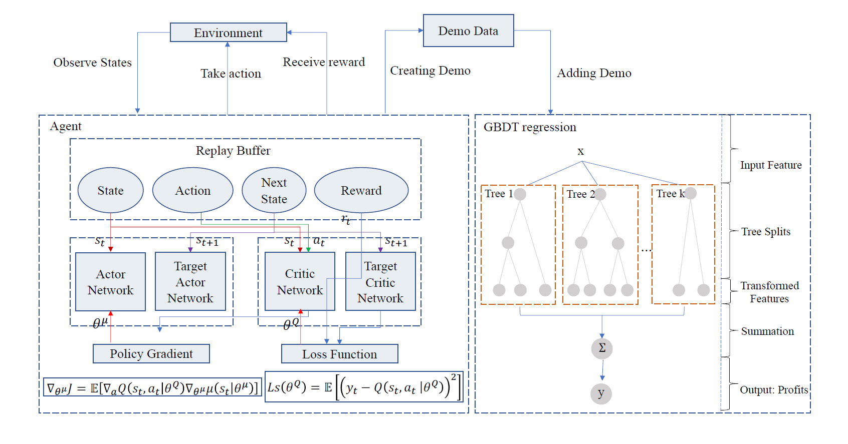
The algorithm of GBDT-based DDPG consists of two steps that are creating demos with the DDPG approach and using a demo which created by the algorithm to train the GBDT model.
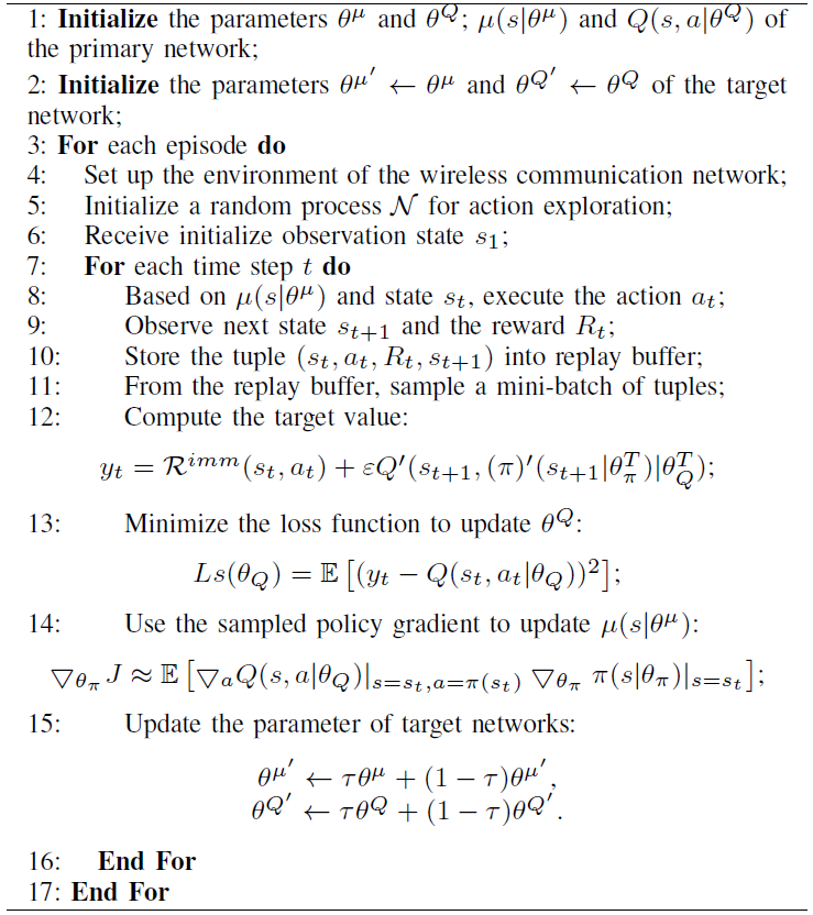
1) Creating demos with the DDPG approach: It is obvious that the training speed of the GBDT model is very fast. However, it cannot learn directly from the environment. DDPG approach can solve the problem that the agent can obtain the maximum return or achieve specific goals through learning optimal strategy in the continuous process of interaction with the environment. However, the GBDT model that is a kind of supervised learning requires correct labels from the environment. Therefore, in our model, we first create an agent through DDPG, and then create a demonstration that contains environment and output reward information. The input data consists of the parameters of the system model ([TeX:] $$F_u, B_u$$, and [TeX:] $$C_u$$) and the parameters of each user [TeX:] $$\Omega_v$$ that include the SINR, the computing ability, the capacity of caching, the content popularity, and the service type requested by the user. The output data includes the amount bandwidth resources [TeX:] $$b_{v_{s_k}, u}$$, computing resources [TeX:] $$f_{v_{s_k}, u}$$, caching resources [TeX:] $$c_{v_{s_k}, u}$$, and the total utility of MVNO. The algorithm of the first step is shown in Algorithm 1.
2) Training the GBDT model using a demo created by DDPG: We use the demo created by DDPG, which consists of environment state, agent action, and reward. Therefore, through continuous training, the GBDT model learns to get the maximal reward for the given environmental information, with the goal of achieving the same level of accuracy as the DRL agent. The algorithm of the second step is shown in Algorithm 2.

VI. SIMULATION RESULTS
This paper uses the environment of Python 3.6 and Tensor- Flow 1.12.0 to simulate and evaluate the performance of the proposed algorithm. In our system, the request of users can be consisted of computation offloading and content caching, and so we set the service-type flag which are “computation offloading request” and “content caching request”. We will randomly choose N users which set the “computation offloading request” flag, and the other M users are set as the flag of “content caching request”. Notably, each user has an unique fixed service request type at each time period t. In this paper, we have selected three types of slices: Bandwidthoriented, computation-oriented, and cache-oriented. In addition, bandwidth-oriented slice refers to services with high bandwidth requirements; computation-oriented slice refers to computation intensive services and cache-oriented slice refers to users that have a large number of tasks that need to be cached. Each slice involves the allocation of three resources. The goal of this paper is to jointly optimize three network resources in these three types of slices.
The total spectral bandwidth of system is set as B = 100 MHz, which can be divided into 1,000 subchannels and the bandwidth of it is [TeX:] $$\mathcal{B}=0.1 \mathrm{MHz}$$. Without loss of generality, the value of SINR in our system can be quantized into five levels, which is {3, 7, 15, 31, 63}, where the value equal to 3 represents very bad wireless channel and the value equal to 31 represents very good wireless channel [39]. In fact, many scholars have already studied the request rate of caching content. Since this article adopts a constant request rate, modeling the request rate of caching content is beyond the scope of this article. Therefore, the Zipf popularity distribution [TeX:] $$p_f$$ is set as the constant which is 0.68.
In order to increase stability of our system, we set two separate target networks, i.e., actor and critic. The learning rate of the actor and critic networks are set as [TeX:] $$\alpha_\theta=0.001$$ and [TeX:] $$\alpha_\omega=0.001$$, respectively. The soft update parameter τ is set as 0.01. In order to train the DNN, we set the values of experience replay buffer and mini-batch to 1,000 and 32. The values of the rest parameters are summarized in Table II.
TABLE II
| Parameters | Value |
|---|---|
| Slice type S | 3 |
| Bandwidth B | 100 MHz |
| Computation capability F | 100 GHz |
| Capacity of cache storage C | 100 GB |
| Computation offloading size of each task | [200,600] Kb |
| Computation capability of each task | [100,200] Megacycles |
| Content size of each task | [5,125] MB |
| Communication rate requirement of each user | 10 Mbps |
| Computation rate requirement of each user | 1 Mbps |
| Energy consumption for one CPU cycle | 1 J/Gegacycles |
| Communication charge [TeX:] $$\lambda_1, \lambda_2, \lambda_3$$ | 50, 40, 60 units/Mbps |
| Computation charge [TeX:] $$\phi_1, \phi_2, \phi_3$$ | 100, 80, 90 units/Mbps |
| Content charge [TeX:] $$\psi_1, \psi_2, \psi_3$$ | 50, 70, 60 units/Mbps |
| Price of communication resource [TeX:] $$\mu_{v_{s_k}, u}$$ | 30 units/MHz |
| Price of computation energy [TeX:] $$\Phi_{v_{s_k}, u}$$ | [TeX:] $$60 \times 10^{-3}$$ units/J |
| Price of the gains of the expected saved backhaul bandwidth [TeX:] $$\Psi_{v_{s_k}, u}$$ | 40 units/MB |
Three schemes are compared with our proposed algorithm, which are the DQN approach, the equal resource allocation (ERA) approach and the random resource allocation (RRA) approach. In order to implement the DQN approach, continuous actions in this paper have been discretized. In addition, two DQN algorithms, i.e., DQN (5-level) and DQN (10-level) indicate that each continuous action is discrete into 5 and 10 levels, respectively.
The convergence performance of the above-mentioned schemes is shown in Fig. 3. It is proved that our proposed scheme is superior to the other comparison methods in terms of MVNO profit and convergence speed. The DDPG-based method comprehensively considers three resource allocation schemes, which can improve the utilization efficiency of network resources and greatly improve the benefits of MVNO. As shown in Fig. 3, at the beginning of the training process, the MVNO profit value of different methods is relatively low. As the number of episodes increased, the MVNO profit of the three different methods reached a stable value after 300 episodes. It is worth mentioning that the agents of DDPG and DQN constantly improve their actions during the first 50 and 70 episodes. After that, the agents of DDPG and DQN explore the nice action-value function at about 50 and 70 episodes, respectively. In fact, the convergence of MVNO profits means that the agent in our proposed system model can continuously learn to obtain the optimal resource allocation strategy.
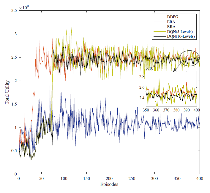
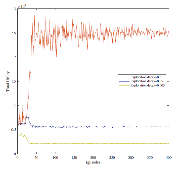
Fig. 4 compares the convergence performance of the DDPG-based algorithm under different exploration decays. In fact, the greater the exploration decay, the greater the randomness of the action. In our simulation, we set the exploration decay to 0.5, 0.05, and 0.005, respectively. As shown in Fig. 4, the greater the exploration decay, the better the profit convergence performance of MVNO. At the same time, a larger exploration decay can speed up the convergence speed of the algorithm. Therefore, the value of exploration decay is set to 0.5 in the remaining simulations.
When the bandwidth, computing and caching resources leased from the InP change, the resources provided by the MVNO to the SP will also change accordingly. As shown in Fig. 5, when the subchannels leased by MVNO increase, more communication resources will be provided to the network slicing, and so the system utility will increase. In the same way, increasing computing ability will make MVNO more profits. When the cache resources leased by MVNO increase, it is expected that more backhaul bandwidth will be saved, and so the revenue of MVNO will increase.
Fig. 5.

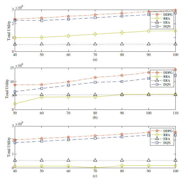
Fig. 6 plots the comparison of the profits of MVNO with respect to the number of task requesters under different schemes. It is obviously that the decrease of MVNO’s profit is approximately linear with the increasing number of computing tasks requested by the user. The reason is that as the number of users requesting computing tasks increases, more users will share the network resources which are composed by computing, caching, and bandwidth. Therefore, the completion of computing tasks causes greater computing delays, resulting in a plummet of MVNO’s utility. However, as the number of users requesting caching tasks increased, the system utility of MVNO will increase. Because caching more content will save more backhaul bandwidth, thereby increasing the revenue of caching. The two subfigures depict that the DDPG algorithm has good performance and surpasses the other comparison algorithms.
Fig. 6.

Fig. 7 shows the total profit of MVNO under different computing, caching, and bandwidth charging prices for different schemes. It can be seen that with the increase of the charging price of computing tasks, the revenue of computing offloading increases. So the agent is more inclined to perform computing offloading to perform user’s computing-intensive tasks. The profit of computation-oriented slice and the total profit of the system are increasing. With the increase of content caching charges, the revenue of caching task has increased, and so the profit of the caching-oriented slice and the total profit of the system are increasing. With the increase of the bandwidth charge, the profit of bandwidth-oriented slice and the total system profit are increasing. It can be seen that the MVNO profit performance of our algorithm is better than other schemes.
Fig. 7.
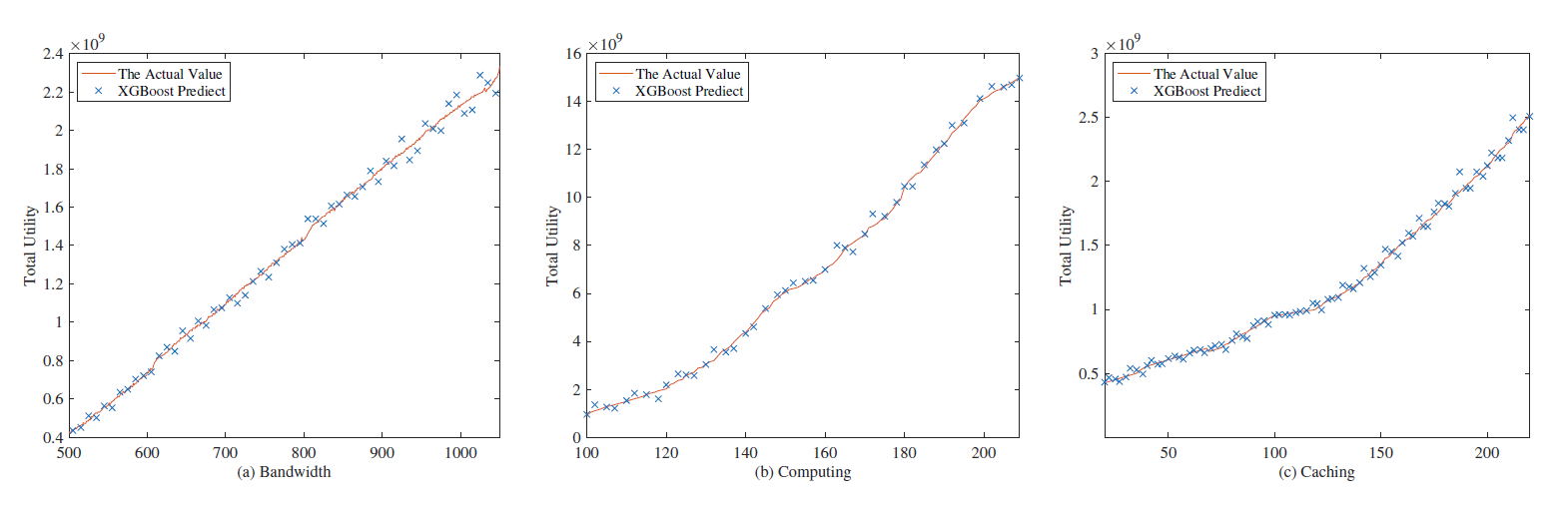
The DDPG algorithm is used to generate a data set of state, action and reward, and then we use the XGBoost model for training. We take the relationship between the total utility of MVNO and the number of subchannels (bandwidth), computing and caching resources leased from InP as an example. The fitting relationship between the predicted result of the XGBoost model and the actual value is shown in Fig. 8. From the figure, we can see that the MVNO revenue predicted by the XGBoost model is basically consistent with the results generated by DDPG. It is proved that the algorithm we proposed is accurate.
After the completion of training, the execution time of the above two algorithms is shown in Table III. Compared with DDPG agents, the GBDT model has obvious advantages in speed. Specifically, with the increase of state space, the speed advantage of GBDT model becomes more prominent.
VII. CONCLUSION
This paper proposes a MEC and caching model that jointly considers communication, computing, and caching resources. The novel profit function is used to measure the performance of MVNO, which takes the revenue of MVNO and the QoE of users into account. Then, we use a DDPG-based edge computing and caching solution. This solution considers the diversity of user service requests and dynamic communication conditions between MEC servers and users to jointly optimize task scheduling and resource allocation in a continuous space. Numerical simulations demonstrate the proposed DDPG algorithm outperforms the other compared algorithms in the literature and achieves the optimal resource allocation scheme. In order to increase the speed of convergence, we use the data set generated by the DDPG algorithm to train the GBDT model. The GBDT model can fully simulate the behavior of DRL agent and the output of results is faster and more costeffective.
Biography
Yu Gong

Yu Gong received the B.S. degree from Jiangxi Normal University in 2018. She is currently studying for a Doctor’s degree in Electronic Science and Technology from Beijing University of Posts and Telecommunications (BUPT). Her current research interests are in intelligent resource allocation strategy, deep reinforcement learning, multi-access edge computing and caching.
Biography
Yifei Wei

Yifei Wei received the B.Sc. and Ph.D. degrees in Electronic Engineering from Beijing University of Posts and Telecommunications (BUPT, China), in 2004 and 2009, respectively. He was a Visiting Ph.D. Student in Carleton University (Canada) from 2008 to 2009. He was a Postdoctoral Research Fellow in the Dublin City University (Ireland) in 2013. He was the Vice Dean of School of Ccience in BUPT from 2014 to 2016. He was a Visiting Scholar in the University of Houston (USA) from 2016 to 2017. He is currently a Professor and the Vice Dean of the School of Electronic Engineering at BUPT. His current research interests are in energy-efficient networking, heterogeneous resource management, machine learning, and edge computing. He is the Guest Editor for a special issue in IEEE Transactions on Green Communications and Networking in 2021. He also served as a symposium Co-Chair of IEEE Globecom 2020, and track Co-Chair for International Conference on Artificial Intelligence and Security (ICAIS) 2019, 2020, 2021 and 2022. He received the best paper awards at the ICCTA2011 and ICCCS2018. He has served on the Technical Program Committee members of numerous conferences.
Biography
F. Richard Yu

F. Richard Yu (Fellow, IEEE) received the Ph.D. de- gree in Electrical Engineering from the University of British Columbia (UBC) in 2003. He joined Carleton University in 2007, where he is currently a Professor. His research interests include connected/autonomous vehicles, security, artificial intelligence, blockchain and wireless cyber-physical systems. He serves on the editorial boards of several journals, including Co-Editor-in-Chief for Ad Hoc Sensor Wireless Networks, Lead Series Editor for IEEE Transactions on Vehicular Technology, IEEE Communications Surveys Tutorials, and IEEE Transactions on Green Communications and Networking. He has served as the Technical Program Committee (TPC) Co-Chair of numerous conferences. He has been named in the Clarivate Analytics list of “Highly Cited Researchers” in 2019 and 2020. He is an IEEE Distinguished Lecturer of both Vehicular Technology Society (VTS) and Comm. Society. He is an elected member of the Board of Governors of the IEEE VTS and Editor-in-Chief for IEEE VTS Mobile World newsletter. Dr. Yu is a registered Professional Engineer in the province of Ontario, Canada, and a Fellow of the IEEE, Canadian Academy of Engineering (CAE), Engineering Institute of Canada (EIC), and Institution of Engineering and Technology (IET).
Biography
Zhu Han

Zhu Han (S’01–M’04-SM’09-F’14) received the B.S. degree in Electronic Engineering from Tsinghua University, in 1997, and the M.S. and Ph.D. degrees in Electrical and Computer Engineering from the University of Maryland, College Park, in 1999 and 2003, respectively. From 2000 to 2002, he was an R Engineer of JDSU, Germantown, Maryland. From 2003 to 2006, he was a Research Associate at the University of Maryland. From 2006 to 2008, he was an Assistant Professor at Boise State Univer- sity, Idaho. Currently, he is with the Department of Electrical and Computer Engineering at the University of Houston, Houston, TX 77004 USA, and also with the Department of Computer Science and Engineering, Kyung Hee University, Seoul, South Korea, 446-701. Dr. Han’s main research targets on the novel game-theory related concepts critical to enabling efficient and distributive use of wireless networks with limited resources. His other research interests include wireless resource allocation and management, wireless communications and networking, quantum computing, data science, smart grid, security and privacy. Dr. Han received an NSF Career Award in 2010, the Fred W. Ellersick Prize of the IEEE Communication Society in 2011, the EURASIP Best Paper Award for the Journal on Advances in Signal Processing in 2015, IEEE Leonard G. Abraham Prize in the field of Communications Systems (best paper award in IEEE JSAC) in 2016, and several best paper awards in IEEE conferences. Dr. Han was an IEEE Communications Society Distinguished Lecturer from 2015-2018, AAAS fellow since 2019, and ACM distinguished Member since 2019. Dr. Han is a 1% highly cited researcher since 2017 according to Web of Science. Dr. Han is also the winner of the 2021 IEEE Kiyo Tomiyasu Award, for outstanding early to mid-career contributions to technologies holding the promise of innovative applications, with the following citation: “for contributions to game theory and distributed management of autonomous communication networks.”
References
- 1 H. Zhang et al., "Network slicing based 5G and future mobile networks: Mobility, resource management, and challenges," IEEE Commun. Mag., vol. 55, no. 8, pp. 138-145, Aug. 2017.doi:[[[10.1109/mcom.2017.1600940]]]
- 2 J. Ordonez-Lucena et al., "Network slicing for 5G with SDN/NFV: Concepts, architectures, and challenges," IEEE Commun. Mag., vol. 55, no. 5, pp. 80-87, May 2017.doi:[[[10.1109/mcom.2017.1600935]]]
- 3 R. Su et al., "Resource allocation for network slicing in 5G telecommunication networks: A survey of principles and models," IEEE Netw., vol. 33, no. 6, pp. 172-179, Nov.-Dec. 2019.doi:[[[10.1109/mnet.2019.1900024]]]
- 4 K. Zhang, S. Leng, Y . He, S. Maharjan, and Y . Zhang, "Cooperative content caching in 5G networks with mobile edge computing," IEEE Wireless Commun., vol. 25, no. 3, pp. 80-87, Jun. 2018.doi:[[[10.1109/mwc.2018.1700303]]]
- 5 Z. Zhou et al., "Social big-data-based content dissemination in Internet of vehicles," IEEE Trans. Industrial Inform., vol. 14, no. 2, pp. 768-777, Feb. 2018.doi:[[[10.1109/tii.2017.2733001]]]
- 6 Z. Ning, X. Wang, and J. Huang, "Mobile edge computing-enabled 5G vehicular networks: Toward the integration of communication and computing," IEEE Veh. Technol. Mag., vol. 14, no. 1, pp. 54-61, Mar. 2019.doi:[[[10.1109/mvt.2018.2882873]]]
- 7 H. Zhu et al., "Caching transient data for Internet of things: A deep reinforcement learning approach," IEEE Internet Things J., vol. 6, no. 2, pp. 2074-2083, Apr. 2019.doi:[[[10.1109/jiot.2018.2882583]]]
- 8 X. Wang et al., "Optimizing content dissemination for real-time traffic management in large-scale Internet of vehicle systems," IEEE Trans. Veh. Technol., vol. 68, no. 2, pp. 1093-1105, Feb. 2019.doi:[[[10.1109/tvt.2018.2886010]]]
- 9 J. Feng et al., "Dynamic network slicing and resource allocation in mobile edge computing systems," IEEE Trans. Veh. Technol., vol. 69, no. 7, pp. 7863-7878, Jul. 2020.doi:[[[10.1109/tvt.2020.2992607]]]
- 10 R. Xie, J. Wu, R. Wang, and T. Huang, "A game theoretic approach for hierarchical caching resource sharing in 5G networks with virtualization," China Commun., vol. 16, no. 7, pp. 32-48, Jul. 2019.doi:[[[10.23919/jcc.2019.07.003]]]
- 11 Z. Li, C. Wang, and C. Jiang, "User association for load balancing in vehicular networks: An online reinforcement learning approach," IEEE Trans. Intell. Transp. Syst., vol. 18, no. 8, pp. 2217-2228, Aug. 2017.doi:[[[10.1109/tits.2017.2709462]]]
- 12 T. P. Lillicrap et al., "Continuous control with deep reinforcement learning," Comput. Sci., Jul. 2019.custom:[[[https://arxiv.org/abs/1509.02971]]]
- 13 T. Hatano et al., "GBDT modeling of deep reinforcement learning agents using distillation," in Proc. IEEE ICM, Mar. 2021.doi:[[[10.1109/icm46511.2021.9385636]]]
- 14 R. Maclin and D. Opitz, "Popular ensemble methods: An empirical study," arXiv e-prints, p. arXiv:1106.0257, Jun. 2011.doi:[[[10.1613/jair.614]]]
- 15 Y . Cheng, J. Zhang, L. Yang, C. Zhu, and H. Zhu, "Distributed green offloading and power optimization in virtualized small cell networks with mobile edge computing," IEEE Trans. Green Commun. Netw., vol. 4, no. 1, pp. 69-82, Mar. 2020.doi:[[[10.1109/tgcn.2019.2949339]]]
- 16 H.-T. Chien, Y .-D. Lin, C.-L. Lai, and C.-T. Wang, "End-to-end slicing with optimized communication and computing resource allocation in multi-tenant 5G systems," IEEE Trans. Veh. Technol., vol. 69, no. 2, pp. 2079-2091, Feb. 2020.doi:[[[10.1109/tvt.2019.2959193]]]
- 17 Y . K. Tun, M. Alsenwi, S. R. Pandey, C. W. Zaw, and C. S. Hong, "Energy efficient multi-tenant resource slicing in virtualized multi-access edge computing," in Proc. APNOMS, Sep. 2019.doi:[[[10.23919/apnoms.2019.8892978]]]
- 18 J. Jankovi´ c, Z. Ili´ c, A. Ora˘ cevi´ c, S. M. A. Kazmi, and R. Hussain, "Effects of differentiated 5G services on computational and radio resource allocation performance," IEEE Trans. Netw. Service Manage., vol. 18, no. 2, pp. 2226-2241, Feb. 2021.doi:[[[10.1109/tnsm.2021.3060865]]]
- 19 X. Chen et al.,, "Optimized computation offloading performance in virtual edge computing systems via deep reinforcement learning," IEEE Internet Things J., vol. 6, no. 3, pp. 4005-4018, Jun. 2019.doi:[[[10.1109/jiot.2018.2876279]]]
- 20 T. Zhang, Z. Wang, Y . Liu, W. Xu, and A. Nallanathan, "Caching placement and resource allocation for cache-enabling UAV NOMA networks," IEEE Trans. Veh. Technol., vol. 69, no. 11, pp. 12897-12911, Nov. 2020.doi:[[[10.1109/tvt.2020.3015578]]]
- 21 L. Lei et al., "Optimal resource allocation for NOMA-enabled cache replacement and content delivery," in Proc. IEEE PIMRC, Sep. 2019.doi:[[[10.1109/pimrc.2019.8904424]]]
- 22 W. Xia and L. Shen, "Joint resource allocation using evolutionary algorithms in heterogeneous mobile cloud computing networks," China Commun., vol. 15, no. 8, pp. 189-204, Aug. 2018.doi:[[[10.1109/cc.2018.8438283]]]
- 23 C. Yi, S. Huang, and J. Cai, "Joint resource allocation for device-todevice communication assisted fog computing," IEEE Trans. Mobile Comput., vol. 20, no. 3, pp. 1076-1091, Mar. 2021.doi:[[[10.1109/TMC.2019.2952354]]]
- 24 L. Zhang, H. Pan, Q. Fan, C. Ai, and Y . Jing, "1GBDT, LR deep learning for turn-based strategy game AI," in Proc. IEEE CoG, Aug. 2019.custom:[[[http://ieeexplore.ieee.org/document/8848103/]]]
- 25 L. Huang and L. Xu, "Research on taxi travel time prediction based on GBDT machine learning method," in Proc. IMCCC, Jul. 2018.doi:[[[10.1109/imccc.2018.00155]]]
- 26 S. Liu, Y . Cui, Y . Ma, and P. Liu, "Short-term load forecasting based on GBDT combinatorial optimization," in Proc. IEEE EI2, Oct. 2018.doi:[[[10.1109/ei2.2018.8582108]]]
- 27 H. Kong, S. Lin, J. Wu, and H. Shi, "The risk prediction of mobile user tricking account overdraft limit based on fusion model of logistic and GBDT," in Proc. IEEE ITNEC, Mar. 2019.doi:[[[10.1109/itnec.2019.8729173]]]
- 28 Y . Luo, J. Yang, W. Xu, K. Wang, and M. D. Renzo, "Power consumption optimization using gradient boosting aided deep Q-network in C-RANs," IEEE Access, vol. 8, pp. 46811-46823, Mar. 2020.doi:[[[10.1109/access.2020.2978935]]]
- 29 Y . Wei, F. R. Yu, M. Song, and Z. Han, "Joint optimization of caching, computing, and radio resources for fog-enabled IoT using natural actorcritic deep reinforcement learning," IEEE Internet Things J., vol. 6, no. 2, pp. 2061-2073, Apr. 2019.custom:[[[https://ieeexplore.ieee.org/document/8513863]]]
- 30 X. Chen, L. Jiao, W. Li, and X. Fu, "Efficient multi-user computation offloading for mobile-edge cloud computing," IEEE/ACM Trans. Netw., vol. 24, no. 5, pp. 2795-2808, Oct. 2016.doi:[[[10.1109/tnet.2015.2487344]]]
- 31 J. Li et al., "Pricing and resource allocation via game theory for a smallcell video caching system," IEEE J. Sel. Areas Commun., vol. 34, no. 8, pp. 2115-2129, Aug. 2016.doi:[[[10.1109/JSAC.2016.2577278]]]
- 32 A. Ndikumana et al., "Joint incentive mechanism for paid content caching and price based cache replacement policy in named data networking," IEEE Access, vol. 6, pp. 33702-33717, Jun. 2018.doi:[[[10.1109/access.2018.2848231]]]
- 33 G. S. Aujla et al., "Data offloading in 5G-enabled software-defined vehicular networks: A stackelberg-game-based approach," IEEE Commun. Mag., vol. 55, no. 8, pp. 100-108, Aug. 2017.doi:[[[10.1109/mcom.2017.1601224]]]
- 34 Z. Ning et al., "Joint computing and caching in 5G-envisioned Internet of Vehicles: A deep reinforcement learning-based traffic control system," IEEE Trans. Intell. Transp. Syst., pp. 1-12, Feb. 2020.doi:[[[10.1109/tits.2020.2970276]]]
- 35 R. Li et al., "Deep reinforcement learning for resource management in network slicing," IEEE Access, vol. 6, pp. 74429-74441, Nov. 2018.doi:[[[10.1109/access.2018.2881964]]]
- 36 R. S. Sutton, D. McAllester, S. Singh, and Y . Mansour, "Policy gradient methods for reinforcement learning with function approximation," Proc. NEURIPS, vol. 12, pp. 1057-1063, Dec. 2000.custom:[[[https://proceedings.neurips.cc/paper/1999/file/464d828b85b0bed98e80ade0a5c43b0f-Paper.pdf]]]
- 37 D. Silver et al., "Deterministic policy gradient algorithms," in Proc. ICML, Jun. 2014.custom:[[[http://proceedings.mlr.press/v32/silver14.pdf]]]
- 38 T. Chen and C. Guestrin, "Xgboost: A scalable tree boosting system," in Proc. ACM SIGKDD, Aug. 2016.doi:[[[10.1145/2939672.2939785]]]
- 39 Y . Wei, Z. Zhang, F. R. Yu, and Z. Han, "Joint user scheduling and content caching strategy for mobile edge networks using deep reinforcement learning," in Proc. IEEE ICC, May 2018.doi:[[[10.1109/iccw.2018.8403711]]]