Time Series Data Cleaning Method Based on Optimized ELM Prediction Constraints

1. Introduction

With the rapid development of the current social economy and information technology, various industries increasingly depend on the acquisition and processing of big data, thus giving rise to the arrival of the era of big data. Time series is a numerical data series that changes with the order of time, and its application field is very wide. It can be applied to many research and business in many fields such as natural science, social science, finance, and economy, so its analysis results are quite important. However, time series may have quality problems in the process of acquisition and preservation, and dirty data exists in large quantities in time series, which will be detrimental to the next step of estimation, clustering, visualization, and other application processing. The purpose of time series cleaning is to detect default values, abnormal values, and timestamp misalignment in the data, fill or repair them, and finally achieve the effect of improving data quality.

There have been many data cleaning methods, but few methods that can be well consumed in time series, so the subsequent rule-based constraints, statistical methods of time series cleaning, and cleaning of time stamps in time series have been produced one after another. Among them, the most representative SCREEN is to use the rate of speed change as a constraint to determine the abnormality of data and then select the repair value according to the median theorem and the principle of minimum change. However, most of these rule-based constraint algorithms use a priori fixed speed change rate as the basis for anomaly detection, and when the abnormal value deviates from the true value by a small amount, it will be considered as correct data and will likely be included in the constraint range. This type of data is difficult to find rule constraint values that can be applied to the entire cleaning process, so this type of cleaning algorithm does not work well over time when the speed change rate between data fluctuates too much.

To address the above-mentioned problem, this paper proposes an online cleaning algorithm that relies on the dynamic speed change rate constraint (CDDC), and how to compute this dynamic speed change rate constraint is the focus of this paper; in order to support online cleaning, a dual-window flow-limiting strategy will be used to partition the two techniques of data cleaning and data prediction, which require a globally optimal solution, into a locally optimal solution for each window. For the problem of dynamic rule constraint solving, after extensive research the extreme learning machine (ELM) algorithm is chosen as the base algorithm for rule constraint prediction, and the optimized ELM algorithm is applied to predict the rate of speed change. Finally, the data points in the detection window are calculated using the dynamic constraint to determine the anomalies.

In order to improve the data repair algorithm, different repair schemes will be used for different types of abnormal point, i.e., intermittent and continuous anomalies [1], to make the repair values closer to the true values. One of them, for intermittent abnormal point repair, the median theorem and the minimum change principle are used to select the final repair solution, transforming the optimal repair solution into a problem of finding an intermediate point and proving that the repair solution for that intermediate point is the optimal repair solution. The other one, for continuous abnormal point repair, the median theorem will no longer be used from the second abnormal point, and the repair solution will be selected based on the orientation of the first anomaly occurring. If it is below the repair value of previous point, the maximum repair scheme will be used, and if it is above the repair value of previous point, the minimum repair scheme will be used.

The following is the main composition of this paper. Section 2 briefly introduces the existing time series data cleaning methods and their problems. Section 3 defines the research problem of time series data cleaning based on dynamic speed constraints, and compares the characteristics and effects of the proposed algorithm with the existing SCREEN algorithm. Section 4 describes the mechanism for implementing stream computing. Section 5 focuses on the process of computing dynamic speed constraints using an optimized ELM. Section 6 details the types of anomalies and their corresponding repair methods.

2. Related Work

Existing widely used filtering cleaning algorithms, such as Kalman filtering [2], nonlinear filtering [3], etc., are used for noise reduction and cleaning of signal data. This cleaning method is based on the regular fixed form of the data to clean the data, which will cause a large part of the correct data to introduce errors.

Smoothing cleaning [4,5] algorithm that can be applied to many fields, for example, SWAB is a stream data cleaning algorithm based on linear interpolation. SMA [6] is a smoothing algorithm used to predict future sequence data based on averages. All smoothing algorithms will also change the correct data in the original sequence.

Statistics-based cleaning algorithm [6-8] calculates the confidence interval of different fields according to statistics to determine abnormal points. The repair strategy in the cleaning algorithm is always determined by the previous data, making the cleaning result unconvincing.

Constraint-based cleaning algorithm [4,5,9-12] establishes constraint rules conforming to historical experience to detect abnormal points according to the characteristic of speed change rate of time series data. Although the optimal repair solution is determined from the repair candidate set, the cleaning ability is improved to a certain extent. However, a constant constraint is set in advance, which makes it unable to process the data with uneven speed fluctuations. Therefore, this paper proposes a cleaning algorithm based on dynamic constraints.

3. Overview

This section defines the problem of the time series data cleaning method based on dynamic speed constraints.

3.1 Problem Description

Form a complete time series data as [TeX:] $$x={{x}}_{[1]}, x_{[2]}, \ldots, x_{[\mathrm{n}]}$$, where the data corresponding to the i-th moment is represented as [TeX:] $$x_{[i]}$$. In order to complete the streaming calculation, the entire time series data is minimally divided by setting a window with a size of w data. For the data in the i-th window, ELM is used to learn the relationship between the past data and speed change rate to predict the speed change rate [TeX:] $$L_{[i]}$$ corresponding to the data contained in the i-th window. In order to accurately detect anomalies, window i needs a maximum value in the loss set obtained from the verification set during the prediction process as the error coefficient , which converts the speed change rate into a speed change range [TeX:] $$\left(s_{[i] \min }\right.,\left.s_{[i] \max }\right)$$, where [TeX:] $$s_{[i] \min }=L_{[i]}-\theta, s_{[i] \max }=L_{[i]}+\theta$$. For the correct data i and j in the same window a, the formula (1) must be satisfied:

Theorem 3.1. When a certain data i cannot satisfy formula (1), it is detected as an abnormal point.

One of the indicators to measure the repair effect is the repair distance, which is the sum of the changes between the sequence to be tested x and repair sequence x', as shown in formula (2):

Theorem 3.2. Each repair value must conform to formula (1), and all repair values are guaranteed to be the minimum value of formula (2).

Another indicator to evaluate the repair effect is the root mean square error (RMS) between the repair value x' and true value r, which is called the loss value:

3.2 Analysis of CDDC and SCREEN

In real life, for data with sharp fluctuations, dynamic speed constraints are better than fixed constraint for data repair. For example, the daily electricity consumption of most family is mainly concentrated at night. For activities at night such as lighting, cooking, watching TV, showering etc., a large number of electrical appliances might work simultaneously, so the changing speed of electricity consumption will increase rapidly. Meanwhile, the change fluctuates greatly because of different electrical appliances with different work and power. During the daytime when only a small number of electrical appliances work, the rate of electricity consumption tends to be constant, and will be much lower than the one at night. If the maximum speed is selected as the speed constraint to repair the electricity consumption data of daytime, only abnormal points with significant deviations can be detected. Actually, existing methods typically choose the maximum speed as the fixed constraints. Although the representative SCREEN algorithm also adopts the window mechanism to assist speed constraint, the speed constraint in this case cannot be applied globally by only adjusting the window size. The reason is that even if the window is set to the minimum (i.e., w = 1), when a large number of users work at the same time, the instantaneous electricity consumption is much higher than the constant speed. Consequently, it is necessary to adopt the dynamic speed constraint. An example is used to illustrate why the changing speed constraint works, where the data is from the household electricity meter data of a residential area.

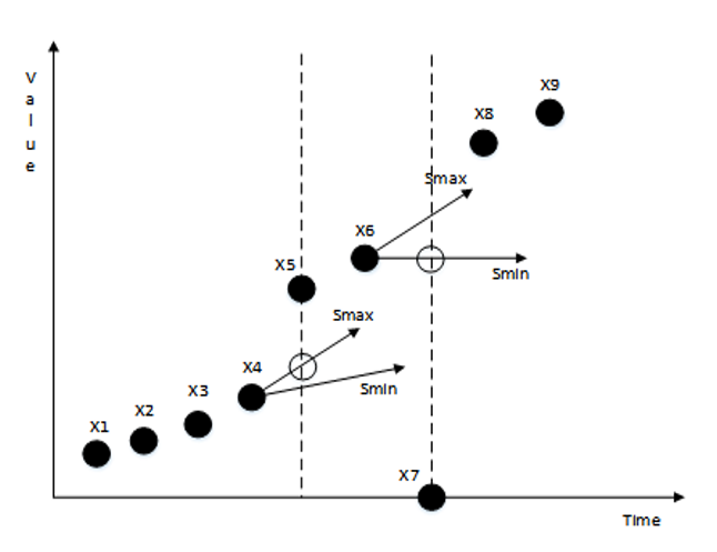
Example 1. Let x = {1.0, 1.5, 2.0, 2.5, 10, 15.0, 0, 30.0, 33.5} to be an original sequence, and suppose its corresponding true value sequence is r={1.0, 1.5, 2.0, 2.5, 3.0, 15.0, 27.5, 30.0, 33.5}, whose timestamp is t = {80, 81, 82, 83, 84, 85, 86, 87, 88}. Let L={0.42, 0.51, 0.49, 0.58, 11.97, 12.59, 2.42, 2.58} be the set of predicted speed constraint with the error coefficient = 0.1 and the window length w = 1. Then, we can obtain a set of constraints s = {(0.32, 0.52), (0.41, 0.61), (0.39, 0.59), (0.48, 0.68), (11.87, 12.07), (12.49, 12.69), (2.32, 2.52), (2.48, 2.68)}. It can be seen that the timestamp distance between data points [TeX:] $$x_{[4]}$$ and [TeX:] $$x_{[5]}$$ in the sequence is [TeX:] $$t_{[5]}-t_{[4]}=1 \leq w$$, and the speed [TeX:] $$\frac{10-2.5}{84-83}=7.5 \notin s_{[4]}$$, similarly, data points [TeX:] $$x_{[6]}$$ and [TeX:] $$x_{[7]}$$ with speed [TeX:] $$\frac{0-15}{87-86}=-15 \notin s_{[6]}$$.

As illustrated in Fig. 1, based on the analysis above, data points [TeX:] $$x_{[5]}$$ and [TeX:] $$x_{[7]}$$ will be considered as points violating constraints that need to be repaired, and the repair results of the two data points are as follows: [TeX:] $$x_{[5]}^{\prime}=2.98, x_{[7]}^{\prime}=27.49$$. Therefore, the repair distance of sequence x is [TeX:] $$\Delta\left(x, x^{\prime}\right)=\sum_{x_{[i]} \in x}\left|x_{[i]}-x_{[i]}^{\prime}\right|=35.97$$, its loss value is RMS = 0.00707.

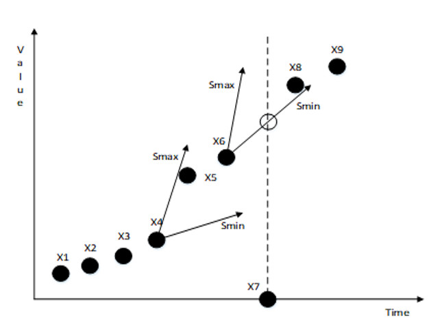
However, if the existing methods like SCREEN are used, the abnormal points cannot be detected. The process is shown in Fig. 2. To ensure the best repair effect of SCREEN, the window length is set to 1. The maximum of the speed [TeX:] $$\left\{\begin{array}{c} s_{\min }=0.5 \\ s_{\max }=12.5 \end{array}\right.$$ is selected as the constraint. Because [TeX:] $$0\lt t_{[5]}-t_{[4]} \leq w$$ and [TeX:] $$0.5 \leq \frac{x_{[5]}-x_{[4]}}{t_{[5]}-t_{[4]}} \leq 12.5$$, as well as the next window is still satisfied the condition [TeX:] $$0\lt t_{[6]}-t_{[5]} \leq w$$ and [TeX:] $$0.5 \leq \frac{x_{[6]}-x_{[5]}}{t_{[6]}-t_{[5]}} \leq 12.5$$, the exception point [TeX:] $$x_{[5]}$$ here is considered to be correct without any repair. Although abnormal point [TeX:] $$x_{[7]}$$ can be detected, their loss value is greater, RMS = 4.33654. Obviously, the proposed CDDC algorithm has a better repair effect.

Fig. 1.

Detection process of CDDC algorithm.

Fig. 2.

Detection process of SCREEN algorithm.

4. Streaming Computing

Data detection and repair often need to obtain a complete sequence. In order to be able to support streaming computing, the window mechanism [9,13] should be considered.

Design a dual-window mechanism consisting of a prediction window and a detection window to achieve simultaneous online prediction and detection of data through streaming computing. First use the data in the historical prediction window as the training set of the machine learning model for training and learning, and then use the data in the next prediction window as the test set to predict the corresponding speed change rate, and always use all the current prediction windows as the training set of the next prediction window to make the predicted value closer to the characteristics of the current time series data, while discarding the data of the first historical prediction window to keep the size of the training set unchanged. Each predicted speed change rate in the prediction window has one and only one corresponding detection window. According to formula (1), the detection window judges whether its data meets the dynamic speed constraint, which is calculated from the speed change rate obtained by the prediction window through the error coefficient θ.

5. Dynamic Speed Constraints

This section will elaborate on how to establish a dynamic constraint model.

5.1 Single Rate of Change

The speed change rate is an index that measures how fast or slow the velocity changes between two data points in unit time. Therefore, considering the characteristics of the speed change rate and the extreme value range based on the change of the speed change rate, a constraint can be calculated to clean the data. For example, if x = {60, 59.33, 76, 57.99, 57.32} is the data of the remaining fuel in the truck's fuel tank at the corresponding timestamp t = {1, 2, 3, 4, 5}, it can be known from experience that fuel consumption cannot be negative and should not more than 0.67 L/min. Therefore, the range of speed change rate is 0–0.67. Obviously, [TeX:] $$x_{[3]}$$ is not within the reasonable range, so it is an abnormal point.

In the scenario above, the data stream usually has relatively stable speed constraint like 0–0.67. However, only applying a constant speed constraint is not enough to detect some abnormal data with subtle changes for data facing large fluctuations in the speed change rate.

5.2 Optimization of ELM Algorithm

ELM is chosen as the neural network model for real-time prediction of speed change rate in order to achieve dynamic speed constraints. On the basis of the original ELM, a secondary prediction strategy is introduced to improve the accuracy of the prediction of the speed change rate. Specifically, it can be described as: train ELM, then put the existing verification set and test set into the trained ELM for testing, and replace the data with poor prediction in the training set with data with better prediction in the verification set, the changed set is used for training again.

Expressed in mathematical form: Suppose [TeX:] $$X=\left\{\left(x_1, y_1\right),\left(x_2, y_2\right), \ldots,\left(x_n, y_n\right)\right\}$$ is the current training sample, and the training sample includes the training set [TeX:] $$X_{\text {train }}=\left\{\left(x_i, y_i\right) \mid i=1,2, \ldots, m\right\}$$ and the validation set [TeX:] $$X_{\text {validation }}=\left\{\left(x_s, y_s\right) \mid s \in(m, n]\right\}(m)$$ two parts, [TeX:] $$Y=\left\{x_1, x_2, \ldots, x_a\right\}$$ are the test samples. First use ELM to learn the training set [TeX:] $$X_{\text {train }}=\left\{\left(x_i, y_i\right) \mid i=1,2, \ldots, m\right\}$$, and respectively predict the training set and the validation set again to obtain [TeX:] $$X_{\text {train }}^{\prime}=\left\{\left(x_i, y_i^{\prime}\right) \mid i=1,2, \ldots, m\right\}$$ and [TeX:] $$X_{\text {validation }}^{\prime}=\left\{\left(x_{\mathrm{s}}, y_{\mathrm{s}}^{\prime}\right) \mid s \in(m, n]\right\}(m \lt n)$$, compare all the prediction results with the real results one by one, and get the loss value set of each predicted data point [TeX:] $$L=\left\{L_i\left|L_i=\right| y_i-y_i^{\prime} \mid, i=1,2, \ldots, n\right\} .$$ When [TeX:] $$x_i=x_s$$, there is

The changed set [TeX:] $$X_{\text {train }}$$ is taken as a training sample for the second training, and the sample Y of the test set is predicted according to the trained prediction model.

5.3 Speed Change Domain

After ELM prediction, the speed change rate of the data points in each window is obtained. Because ELM is a single hidden layer neural network, even after improvement, its prediction result is still difficult to be completely equal to the true value, so the speed change rate cannot be used to directly clean the data as a constraint. Compared with a single point value, it is more inclined to use the threshold value as a constraint in the cleaning process, that is, the speed change rate is mapped into an interval through the error coefficient as the speed change domain [TeX:] $$s_i\left(s_{[i] \min }, s_{[i] \max }\right)$$. The calculation of the error coefficient [TeX:] $$\theta =\max \left(L_{\text {validation }}\right)$$ is the loss value set [TeX:] $$L_{\text {validation }}=\left\{L_i \mid L_1, L_2, \ldots, L_n\right\}$$ obtained from the prediction results of the current validation set to determine its maximum value according to the minimum change principle as the error coefficient θ. The calculation formula of the speed change domain is:

6. Data Repair

The repair in traditional methods represented by SCREEN [14] is only effective for intermittent abnormal points. This section proposes effective repair methods for consecutive abnormal data and provides theoretical proofs.

6.1 Repair of A Single Abnormal Point

For a single abnormal point [TeX:] $$x_k,$$ based on the relationship with other data points after [TeX:] $$x_k$$ in the window n, the dynamic rule is used as the constraint condition for repair, and the median theorem is used to determine that [TeX:] $$x_k^{\text {mid }}$$ in the set of repair candidates [TeX:] $$\left(X_k^{\min } \cup X_k^{\max } \cup\left\{x_k\right\}\right)$$ is the optimal repair value, and the calculation formula of the repair candidate value is expressed as:

(6)

[TeX:] $$\begin{aligned} X_k^{\min } =\left\{x_i+s_{[i] \min }\left(t_k-t_i\right) \mid t_k \lt t_i \lt t_k+w, 1 \leq i \leq n\right\} \\ X_k^{\max } =\left\{x_i+s_{[i] \max }\left(t_k-t_i\right) \mid t_k \lt t_i \lt t_k+w, 1 \leq i \leq n\right\} \end{aligned}$$

According to [TeX:] $$x_{k-1}^{\prime}$$ that has been repaired before, another repair candidate set of [TeX:] $$\mathcal{x}_k$$ can be determined, that is, the optimal repair value determined by formula (6) should be included in the repair candidate range [TeX:] $$\left[x_k^{\min }, x_k^{\max }\right]$$ calculated by [TeX:] $$x_{k-1}^{\prime}$$, where

(7)

[TeX:] $$\begin{aligned} x_k^{\min } =x_{k-1}^{\prime}+s_{[i] \min }\left(t_k-t_{k-1}\right) \\ x_k^{\max } =x_{k-1}^{\prime}+s_{[i] \max }\left(t_k-t_{k-1}\right) \end{aligned}$$

Based on the monotonicity of the function, once [TeX:] $$x_k^{\text {mid }} \notin\left[x_k^{\text {min }}, x_k^{\max }\right],$$ the formula for calculating the optimal repair value is as follows:

(8)

[TeX:] $$x_k^{\prime}=\left\{\begin{array}{l} x_k^{\max } x_k^{\max } \lt x_k^{\operatorname{mid}} \\ x_k^{\min } x_k^{\min } \gt x_k^{\operatorname{mid}} \\ x_k^{\operatorname{mid}} \text { otherwise } \end{array}\right.$$

6.2 Repair of Consecutive Null Value Abnormal Points

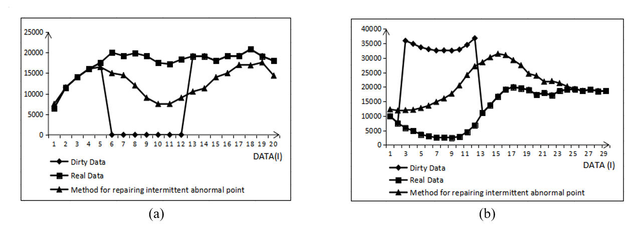
It is stipulated that as long as it is satisfied that when [TeX:] $$x_k$$ is an abnormal point and [TeX:] $$x_{k-1}^{\prime} \neq x_{k-1}, x_k$$ is always less than [TeX:] $$x_{k-1}^{\prime}$$, then [TeX:] $$x_{k-1}$$ to [TeX:] $$x_k$$(1 k n) are called consecutive null value abnormal points, until [TeX:] $$x_{k+n}=\operatorname{median}\left(X_{k+n}{ }^{\min } \cup X_{k+n}{ }^{\max } \cup\left\{x_{k+n}\right\}\right)$$ appears, then [TeX:] $$x_{k+n}$$ is the correct point, and the consecutive abnormal point ends. It can be seen from Fig. 3(a) that for the abnormal points with consecutive null values, once the repair method of a single abnormal point is applied, the smallest number in the candidate set is always regarded as the optimal repair value, so the repair value will continue to show a downward trend within a period of time, causing a greater deviation from the true value. In addition, when the abnormal data point ends and the correct data point arrives, the method will also repair the correct data point, and slowly approach the true value after a long time. Since the repair method of a single abnormal point is based on minimum change principle, that is, in the process of repairing consecutive null values, the smallest number in the candidate set is always used as the repair value. Therefore, we believe that if the largest number in the candidate set is used as the repair value when the second null value is encountered, the repair value will be closer to the true value faster. So in the repair process, we set a condition, that is, after the value of [TeX:] $$x_{k-1}$$ is changed, if the data point [TeX:] $$x_k$$ is still an abnormal point, and [TeX:] $$x_k \lt x_{k-1}^{\prime}$$, then [TeX:] $$x_k^{\prime}=x_{k-1}{ }^{\max }, \text { where } x_{k-1}{ }^{\max } \in\left[x_{k-1}{ }^{\min }, x_{k-1}{ }^{\max }\right].$$

6.3 Repair of Consecutive Normal Value Abnormal Points

If [TeX:] $$x_k$$ is a consecutive abnormal point and is always greater than [TeX:] $$x_{k-1}^{\prime}$$, then [TeX:] $$x_{k-1}$$ to [TeX:] $$x_k(1 \lt k \lt n)$$ are called consecutive normal value abnormal points and need to be repaired until [TeX:] $$x_{k+n}=x_{k+n}^{\prime},$$ indicating that the consecutive abnormal point ends. Contrary to the idea of repairing consecutive null abnormal points, when repairing the second consecutive normal abnormal point in Fig. 3(b), a judgment condition should also be added, that is, after [TeX:] $$x_{k-1}$$ is repaired, if the data point [TeX:] $$x_k$$ is still regarded as an abnormal point, and [TeX:] $$x_k>x_{k-1}^{\prime}, \text { then } x_k^{\prime}=x_{k-1}{ }^{\min }, \text { where } x_{k-1}{ }^{\min } \in\left[x_{k-1}{ }^{\min }, x_{k-1}{ }^{\max }\right] \text {. }$$

Fig. 3.

Comparison of repair effects: (a) repair effect of consecutive null value abnormal points and (b) repair effect of consecutive normal value abnormal points.

6.4 Effectiveness of Repairing Consecutive Abnormal Points

We formally describe the effectiveness of the improved repair method for consecutive anomaly and the final experiment also verify this.

In order to further demonstrate the reliability of the improved repair method for consecutive null abnormal points, the deviation of the traditional single abnormal point repair method is compared. As shown in Fig. 3(a), data points [TeX:] $$x_1-x_5$$ do not need to be repaired and the detection window size is assumed to be 3. Therefore, when [TeX:] $$x_6$$ is determined as an abnormal point, [TeX:] $$x_5$$ is calculated as the candidate repair set of [TeX:] $$x_6$$ that is: [TeX:] $$x_6{ }^{\text {max }}=x_5{ }^{\prime}+s_{max}(t_6-t_5)=x_5{ }^{\prime}+s_{max}; x_6{ }^{\text {min }}=x_5{ }^{\prime}+s_{min}(t_6-t_5)=x_5{ }^{\prime}+s_{min}.$$ According to the data points [TeX:] $$x_7, x_8$$ and formula (6), [TeX:] $$x_6{}^{\operatorname{mid}}=\operatorname{median}\left(\left\{X_6{}^{\max }\right\} \cup\left\{X_6{}^{\min }\right\} \cup x_6\right)=0$$. Because of [TeX:] $$x_6{}^{\text {mid }}\lt x_6{}^{\min }$$, so [TeX:] $$x_6{}^{\prime}=x_5{ }^{\prime}+s_{\text {min }}$$. According to the above steps, if there are n consecutive null value abnormal points, then the repair value of the n-th consecutive null value abnormal point [TeX:] $$x_n{}^{\prime}=x_5{}^{\prime}+(n-5) s_{\text {min }}$$. Now, let us consider the case of using the proposed method of repairing consecutive null value abnormal points. There is still no need to repair [TeX:] $$x_1-x_5$$. The repair steps of [TeX:] $$x_6$$ are the same as in the traditional method, namely [TeX:] $$x_6{}^{\prime}=x_5{}^{\prime}+s_{\text {min }}$$. When the next point [TeX:] $$x_7$$ is still an abnormal point, and [TeX:] $$x_7 \lt x_6{}^{\prime}$$, then [TeX:] $$x_7{}^{\prime} = x_6{}^{\prime}+s_{max} = x_5{}^{\prime}+s_{min}+s_{\max}$$. In the same way, it can be deduced that the repair value of the n-th consecutive null value abnormal point should be [TeX:] $$x_n{}^{\prime}=x_5{}^{\prime}+(n-6) s_{\max }+s_{\text {min }}.$$ Thus for traditional method: [TeX:] $$x_n{}^{\prime}=x_5{}^{\prime}+(n-5) s_{\text {min }}=x_5{}^{\prime}+(n-5)L_{[i]}-(n-5)\theta,$$ while for the improved consecutive null value repair method, [TeX:] $$x_n{}^{\prime}=x_5{}^{\prime}+(n-6) s_{\text {max}}+s_{\text {min }}=x_5{}^{\prime}+(n-5)L_{[i]}+(n-7)\theta.$$

When the traditional single abnormal point repair method is used to repair the abnormal point of continuous normal value, [TeX:] $$x_n{}^{\prime}=x_2{}^{\prime}+(n-2) s_{\text {max}}=x_2{}^{\prime}+(n-2)L_{[i]}+(n-2)\theta;$$ an improved method of repairing consecutive normal value abnormalities is applied, then [TeX:] $$x_n{}^{\prime}=x_2{}^{\prime}+(n-2)L_{[i]}-(n-4)\theta.$$

Comparing the deviations produced by repairing two kind of consecutive abnormal points through the traditional method and the improved method respectively shows that the accuracy of the improved method of repairing consecutive abnormal points is always higher by 2θ.

7. Experiment

In this section, the performance of the proposed method CDDC is evaluated according to several groups of experiments based on real datasets. The effectiveness and stability of CDDC are tested mainly by controlling the size of datasets and abnormal proportion.

7.1 Environment Configuration

The entire experiment will be conducted on a PC with the following configuration: 32 GB RAM, Core i7-8750H 2.20 GHz CPU, Windows 10 operating system. Java language is used for implementation. The dataset used is the New York cab usage dataset, this public dataset is easier to obtain compared to such datasets as electricity meter data, aircraft flight parameters, etc., at the same time, it is similar to the above difficult to obtain datasets in terms of data fluctuation and has a certain representativeness, so it is chosen to represent most of the data with uneven speed change as the dataset for this experiment.

7.2 Evaluation of Cleaning Methods

This section mainly compares the cleaning method CDDC proposed in this paper with the traditional cleaning method SCREEN on a representative public dataset, and proves that the former has a better effect on cleaning time series data.

In order to have a certain data prediction ability, we first analyze and compare the current popular machine learning methods from two aspects of loss value RMS and time cost [15,16]. As shown in Fig. 4(a) and 4(b), the loss values of Back propagation neural network (BP neural network) [17], extreme learning machine with forgetting mechanism (FOS-ELM) [18], extreme learning machine with online (OR-ELM), variants of extreme learning machine with online (NFOS-ELM) are at the peak when the dataset size is 192, 94, 384, and 672, respectively, that is, when the dataset is small, the prediction effect of the above model is poor. As for NAOS-ELM, although its loss value is always low, it cannot be applied to our algorithm because the prediction effect fluctuates too much. Only the loss value predicted by ELM as a whole is in the acceptable range and has the lowest time consumption. It is worth mentioning that the larger the dataset, the smaller the time cost required, so ELM better meets our requirements for data prediction.

Based on the concept of the validation set, the ELM is optimized by quadratic prediction, which achieved more accurate data prediction, and the effectiveness of the optimization is proved through experiments. The optimized ELM in Fig. 4(c) is always lower than the original ELM in terms of loss value. Moreover, when the training set is small, the optimized ELM predicts better. As shown in Fig. 4(d), when the dataset is small, there is little difference in time between the two algorithms; when the dataset is large, although the optimized ELM consumes slightly more time than the original ELM, the predicted delay is within a reasonable range.

Fig. 4.

Comparison of the effect of data prediction: (a) error of prediction models, (b) time cost of error of prediction models, (c) error of ELM and its optimization, and (d) time cost of ELM and its optimization.

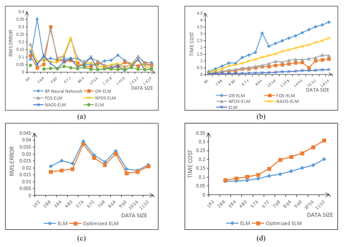
Fig. 5(a) plots the curve of the accuracy of data detection between the CDDC proposed in this paper and the traditional approach SCREEN [19]. Comparing the two shows that the CDDC has a better detection effect on abnormal points; Fig. 5(b) shows that although the blue curve representing the time consumed by CDDC is always above the yellow curve representing the time cost of SCREEN, and the larger the dataset, the more time it consumes, but this is because the optimized ELM requires one more training. The overall time-consuming is large, which can be solved by window adjustment. Therefore, CDDC still has a higher cleaning capacity.

Fig. 5.

Performance comparison of CDDC and SCREEN: (a) accuracy comparison of CDDC and SCREEN and (b) time cost comparison of CDDC and SCREEN.

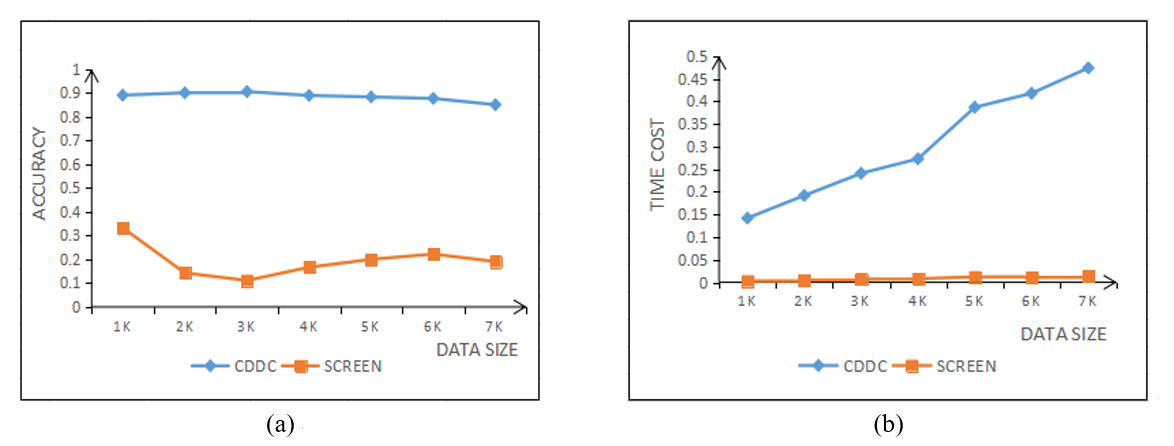
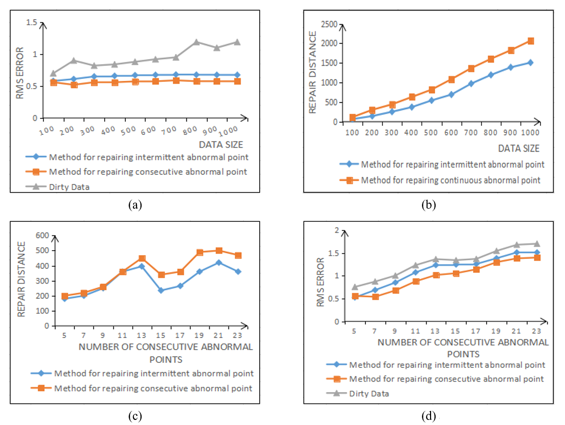
Fig. 6(a) and 6(d) and Fig. 6(b) and 6(c) compare and describe the two indexes of loss value and repair distance between the improved repair method and the traditional repair method [20] from the perspective of the size of dataset and the proportion of abnormal points. The experimental results show that the improved method can repair the consecutive abnormal points more accurately.

Fig. 6.

Comparison between improved repair methods and traditional repair methods: (a) error of improved repair method and traditional repair method under different data size, (b) repair distance of improved repair method and traditional repair method under different data size, (c) error of improved repair method and traditional repair method under different abnormal ratios, and (d) repair distance of improved repair method and traditional repair method under different abnormal ratios.

8. Process of Algorithm

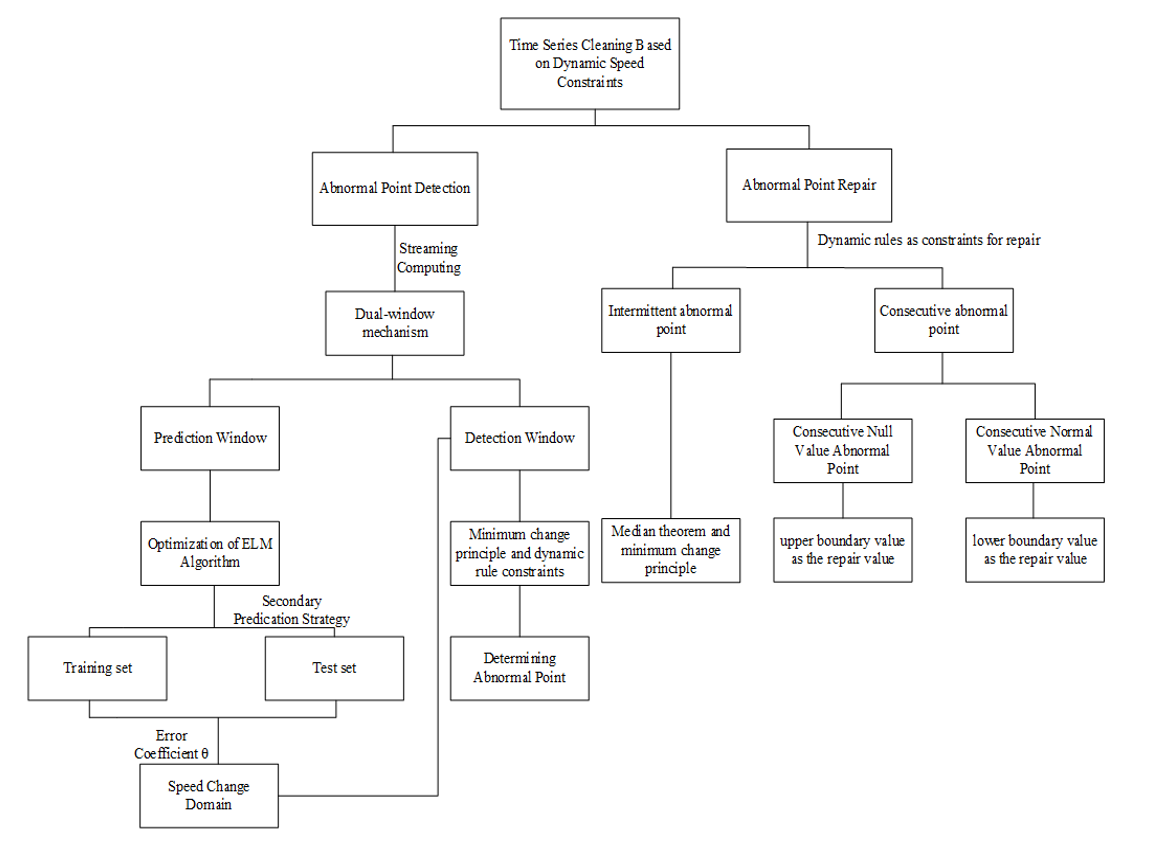
Due to the limited space of the paper, some specific steps cannot be reflected in the paper. In order to make readers understand and reproduce, the modules, steps and processes of CDDC algorithm implementation are provided here, as shown in Fig. 7.

Fig. 7.

Overview of the CDDC algorithm.

References

- 1 M. V olkovs, F. Chiang, J. Szlichta, and R. J. Miller, "Continuous data cleaning," in Proceedings of 2014 IEEE 30th International Conference on Data Engineering, Chicago, IL, 2014, pp. 244-255.doi:[[[10.1109/icde.2014.6816655]]]
- 2 M. S. Grewal, A. P . Andrews, and C. G. Bartone, "Kalman filtering," in Global Navigation Satellite Systems, Inertial Navigation, and Integration, 4th ed. Hoboken, NJ: John Wiley Sons Inc., 2020, pp. 355-417.custom:[[[-]]]
- 3 A. Harvey, K. Laskey, and K. C. Chang, "Machine learning applications for sensor tasking with non-linear filtering," 2021 (Online). Available: https://www.researchgate.net/publication/350358429_Machine_Learning_ Applications_for_Sensor_Tasking_with_Non-Linear_Filtering.custom:[[[https://www.researchgate.net/publication/350358429_Machine_Learning_Applications_for_Sensor_Tasking_with_Non-Linear_Filtering]]]
- 4 A. Nielsen, Practical Time Series Analysis: Prediction with Statistics and Machine Learning. Sebastopol, CA: O'Reilly Media, 2019.custom:[[[https://www.oreilly.com/library/view/practical-time-series/9781492041641/]]]
- 5 H. Li, "Time works well: dynamic time warping based on time weighting for time series data mining," Information Sciences, vol. 547, pp. 592-608, 2021.doi:[[[10.1016/j.ins.2020.08.089]]]
- 6 M. H. P . Swari, I. P . S. Handika, and I. K. S. Satwika, "Comparison of simple moving average, single and modified single exponential smoothing," in Proceedings of 2021 IEEE 7th Information Technology International Seminar (ITIS), Surabaya, Indonesia, 2021, pp. 1-5.doi:[[[10.1109/itis53497.2021.9791516]]]
- 7 W. Li, L. Li, Z. Li, and M. Cui, "Statistical relational learning based automatic data cleaning," Frontiers of Computer Science, vol. 13, no. 1, pp. 215-217, 2019.doi:[[[10.1007/s11704-018-7066-4]]]
- 8 H. Ren, B. Xu, Y . Wang, C. Yi, C. Huang, X. Kou, et al. "Time-series anomaly detection service at Microsoft," in Proceedings of the 25th ACM SIGKDD International Conference on Knowledge Discovery Data Mining, Anchorage, AK, 2019, pp. 3009-3017.doi:[[[10.1145/3292500.3330680]]]
- 9 M. Khatami and F. Akbarzadeh, "Algorithms for segmenting time series," Global Analysis and Discrete Mathematics, vol. 3, no. 1, pp. 65-73, 2018.custom:[[[https://gadm.du.ac.ir/article_128_d7612e93083ec09c04afda52b814a71e.pdf]]]
- 10 X. Wang and C. Wang, "Time series data cleaning with regular and irregular time intervals," 2020 (Online). Available: https://arxiv.org/abs/2004.08284.custom:[[[https://arxiv.org/abs/2004.08284]]]
- 11 A. A. Alzou’bi and K. H. Gan, "Discovering informative features in large-scale landmark image collection," Journal of Information Science, vol. 48, no. 2, pp. 237-250, 2022.doi:[[[10.1177/0165551520950653]]]
- 12 X. Wang and C. Wang, "Time series data cleaning: a survey," IEEE Access, vol. 8, pp. 1866-1881, 2019.doi:[[[10.1109/access.2019.2962152]]]
- 13 M. M. Liu, Q. C. Hu, J. F. Guo, and J. Chen, "Link prediction algorithm for signed social networks based on local and global tightness," Journal of Information Processing Systems, vol. 17, no. 2, pp. 213-226, 2021.doi:[[[10.3745/JIPS.04.0210]]]
- 14 R. P . Shetty, A. Sathyabhama, and P . S. Pai, "An efficient online sequential extreme learning machine model based on feature selection and parameter optimization using cuckoo search algorithm for multi-step wind speed forecasting," Soft Computing, vol. 25, pp. 1277-1295, 2021.doi:[[[10.1007/s00500-020-05222-x]]]
- 15 G. B. Huang, Q. Y . Zhu, and C. K. Siew, "Extreme learning machine: a new learning scheme of feedforward neural networks," in Proceedings of 2004 IEEE International Joint Conference on Neural Networks (IEEE Cat. No. 04CH37541), Budapest, Hungary, 2004, pp. 985-990.doi:[[[10.1109/ijcnn.2004.1380068]]]
- 16 S. Huang, B. Wang, Y . Chen, G. Wang, and G. Y u, "An efficient parallel method for batched OS-ELM training using MapReduce," Memetic Computing, vol. 9, pp. 183-197, 2017.doi:[[[10.1007/s12293-016-0190-5]]]
- 17 R. Hecht-Nielsen, "Theory of the backpropagation neural network," in Proceedings of the International Joint Conference on Neural Networks, Washington, DC, 1989.doi:[[[10.1109/ijcnn.1989.118638]]]
- 18 D. Lahoz, B. Lacruz, and P . M. Mateo, "A multi-objective micro genetic ELM algorithm," Neurocomputing, vol. 111, pp. 90-103, 2013.doi:[[[10.1016/j.neucom.2012.11.035]]]
- 19 S. Song, A. Zhang, J. Wang, and P . S. Y u, "SCREEN: stream data cleaning under speed constraints," in Proceedings of the 2015 ACM SIGMOD International Conference on Management of Data, Melbourne, Australia, 2015, pp. 827-841.doi:[[[10.1145/2723372.2723730]]]
- 20 P . Bohannon, W. Fan, M. Flaster, and R. Rastogi, "A cost-based model and effective heuristic for repairing constraints by value modification," in Proceedings of the 2005 ACM SIGMOD International Conference on Management of Data, Baltimore, MD, 2005, pp. 143-154.doi:[[[10.1145/1066157.1066175]]]
- 21 J. V an den Broeck and L. T. Fadnes, "Data cleaning," Epidemiology: Principles and Practical Guidelines. Dordrecht, Netherlands: Springer, 2013, pp. 389-399.doi:[[[10.1007/978-94-007-5989-3]]]
- 22 D. Cervo and M. Allen, Master Data Management in Practice: Achieving True Customer MDM. Hoboken, NJ: John Wiley Sons, 2011.custom:[[[https://www.wiley.com/en-us/Master+Data+Management+in+Practice:+Achieving+True+Customer+MDM-p-9780470910559]]]
- 23 H. Liu, A. K. Tk, J. P . Thomas, and X. Hou, "Cleaning framework for bigdata: an interactive approach for data cleaning," in Proceedings of 2016 IEEE Second International Conference on Big Data Computing Service and Applications (BigDataService), Oxford, UK, 2016, pp. 174-181.doi:[[[10.1109/bigdataservice.2016.41]]]
- 24 M. S. Chen, J. Han, and P . S. Y u, "Data mining: an overview from a database perspective," IEEE Transactions on Knowledge and data Engineering, vol. 8, no. 6, pp. 866-883, 1996.doi:[[[10.1109/69.553155]]]
- 25 L. Wang, L. D. Xu, Z. Bi, and Y . Xu, "Data cleaning for RFID and WSN integration," IEEE Transactions on Industrial Informatics, vol. 10, no. 1, pp. 408-418, 2014.doi:[[[10.1109/tii.2013.2250510]]]
- 26 X. Shen, X. Fu, and C. Zhou, "A combined algorithm for cleaning abnormal data of wind turbine power curve based on change point grouping algorithm and quartile algorithm," IEEE Transactions on Sustainable Energy, vol. 10, no. 1, pp. 46-54, 2019.doi:[[[10.1109/tste.2018.2822682]]]