Link Budget Analysis for Inter-Satellite FSO Links with Comprehensive Pointing-Error Models

Ⅰ. Introduction

In recent years, Low-Earth-Orbit (LEO) satellite constellations have attracted significant attention for providing global broadband services with reduced latency and improved coverage^[1,2]. A key component of these constellations is the inter-satellite link (ISL), which enables satellites to communicate directly with one another,thereby minimizing reliance on ground stations and enhancing overall network robustness^[3]. Among various ISL technologies, free-space optical (FSO) communication shows particular promise due to its high data rate potential,low power consumption, and resistance to radio-frequency interference^[4]. However,FSO ISLs remain vulnerable to jitter, which can lead to beam misalignment and severely impact link performance. To address this challenge, we derive the probability density functions (PDFs) for pointing errors using the relationship between pointing-error radial displacement and pointing error. Next, we determine a realistic ISL distance by applying a specific SpaceX Starlink constellation model. Finally, utilizing these results, we analyze the ISL link budget using closed-form and Monte Carlo simulation methods over varying jitter levels under a given power constraint.

ISL can be implemented using either radio-frequency (RF) technology or free-space optical (FSO) systems. FSO communication employs signals in the nanometer wavelength range, which is significantly shorter than the wavelengths used in RF systems. Recently, FSO-based ISLs have emerged as a transformative technology owing to numerous advantages over their RF counterparts, including higher bandwidth, smaller antenna size (approximately one-tenth the diameter of RF antennas), greater directivity due to narrower beam divergence (around one-thousandth that of RF), enhanced power efficiency (roughly twice that of RF), operation in an unlicensed spectrum band, and improved security^[5,6]. The narrow beam divergence also underscores the importance of precisely aligning the transmitter and receiver.

When deploying and maintaining FSO ISLs, pointing, acquisition, and tracking (PAT) terminals play a critical role^[7]. Specifically, pointing involves accurately aiming the laser beam at the PAT terminal of a neighboring satellite, acquisition entails pinpointing the satellite’s location and initializing the ISL connection, and tracking continuously monitors the relative positions of the satellites to maintain a stable and reliable link. During pointing, two primary types of misalignment can arise: transmitter pointing error and receiver pointing error. Both reduce overall link efficiency by causing pointing losses, making it essential to quantify and model their effects.

Several statistical models describing pointing errors ―based on the radial displacement between the receiver aperture center and the actual beam spot―have been examined in [8]. In [9], three of these models were selected for a more in-depth analysis of the statistical channel in ship-to-ship(orship-to-shore) links, resulting in an integrated channel model. These studies mainly investigated either the ergodic capacity of the models^[8] or the average bit error rate(BER)^[9] as a function of the average signal-to-noise ratio (SNR).

In this paper, we first derive six probability density function (PDF) models of pointing error, covering all potential scenarios that may arise from satellite vibrations and orientation changes. We then compute the expected pointing loss. Finally, we analyze the link budget for these six models under different jitter levels, using five realistic ISL distances. The remainder of this paper is organized as follows: Section Ⅱ presents the system and channel models, focusing on the pointing-error PDFs and the ISL link distance. In Section Ⅲ, we analyze the link budget, and numerical results are discussed in Section Ⅳ. Section Ⅴ concludes the paper.

Ⅱ. System and Channel Model

2.1 System Model

In the additive white Gaussian noise (AWGN) channel,the received signal y can be expressed as

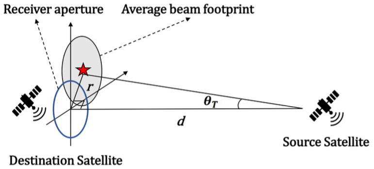
where η is the effective photoelectric conversion ratio, x is the transmitted signal, h is the channel gain and n is the additive white Gaussian noise with variance N₀. In FSO communication, the channel gain h is typically modeled as h=h_lh_ah_p, where h_lis the atmospheric loss factor, h_a is the atmospheric fading factor, and h_p is the pointing error factor. In case of inter-satellite link where the communication takes place in space, the atmospheric effect can be neglected, so the channel gain h can be simplified as h_p.

2.2 Pointing-Error Radial Displacement Statistical Model

Pointing error in FSO communication is typically characterized by two main elements: boresight and jitter. Fig. 1 describes the motion of the beam and the position of boresight and jitter. As satellites move along the orbit, subtle turbulence causes the beam alignment between the transmitter and the receiver to shiver and yields lots of instantaneous beam footprints. The boresight is the fixed radial displacement between the receiver aperture and the average beam footprint where its displacement and coordinate are expressed as r and(μ_x, μ_y) in the cartesian coordinate system, respectively^[9]. Jitter is the random offset of the beam center and expressed in σ_x for x-axis and σ_y for y-axis.

Fig. 1.

Beam’s motion and the positions of the boresight and jitter are illustrated. Red star indicates the boresight, w _z denotes the beamwidth, r is the radial displacement caused by pointing error, and a represents the receiver aperture radius. Jitter along the x- and y-axes are denoted by σ _x and σ _y, respectively.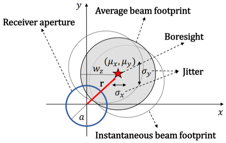

Assuming a Gaussian beam, the collected power at the receiver aperture can be approximated as

where z is the link distance, [TeX:] $$A_0=[\operatorname{erf}(v)]^2$$ is the maximum fraction of the collected power where r=0, [TeX:] $$v=\sqrt{\frac{a^2 \pi}{2 w_z^2}}$$ is the ratio between the receiver aperture radius a and the beamwidth w_z where [TeX:] $$\operatorname{erf}(x)=\frac{2}{\sqrt{\pi}} \int_0^x e^{-t^2} d t$$ is the error function. The approximation made in (2) is valid only under the condition where w_z>6a. The equivalent beamdwidth is expressed as [TeX:] $$w_{z_{q q}}=\sqrt{w_z^2 \frac{\sqrt{A_0 \pi}}{2 v \exp \left(-v^2\right)}}$$. Noticing the fact that the beam is Gaussian, radial displacement vector r can be written as [TeX:] $$\mathbf{r}=\left[\begin{array}{ll} r_x & r_y \end{array}\right]^T$$ where r_x and r_y follow independent Gaussian distribution as [TeX:] $$r_x \sim N\left(\mu_x, \sigma_x^2\right)$$ and [TeX:] $$r_y \sim N\left(\mu_y, \sigma_y^2\right)$$, respectively. Accordingly, the radial displacement can be expressed as [TeX:] $$r=|\mathbf{r}|=\sqrt{r_x^2+r_y^2}$$.

According to the characteristic of boresight and jitter, the pointing-error radial displacement models can be classified into six different distributions as described below. The Gaussian beam footprint and the probability density function (PDF) of each cases are shown in Fig. 2 and Table 1, respectively.

Fig. 2.

Comprehensive six different pointing-error radial displacement models such as: (a) Beckmann distribution, (b) Rayleigh distribution, (c) Rician distribution, (d) Hoyt distribution, (e) Zero-mean single-sided Gaussian distribution, (f) Non-zero mean single-sided Gaussian distribution.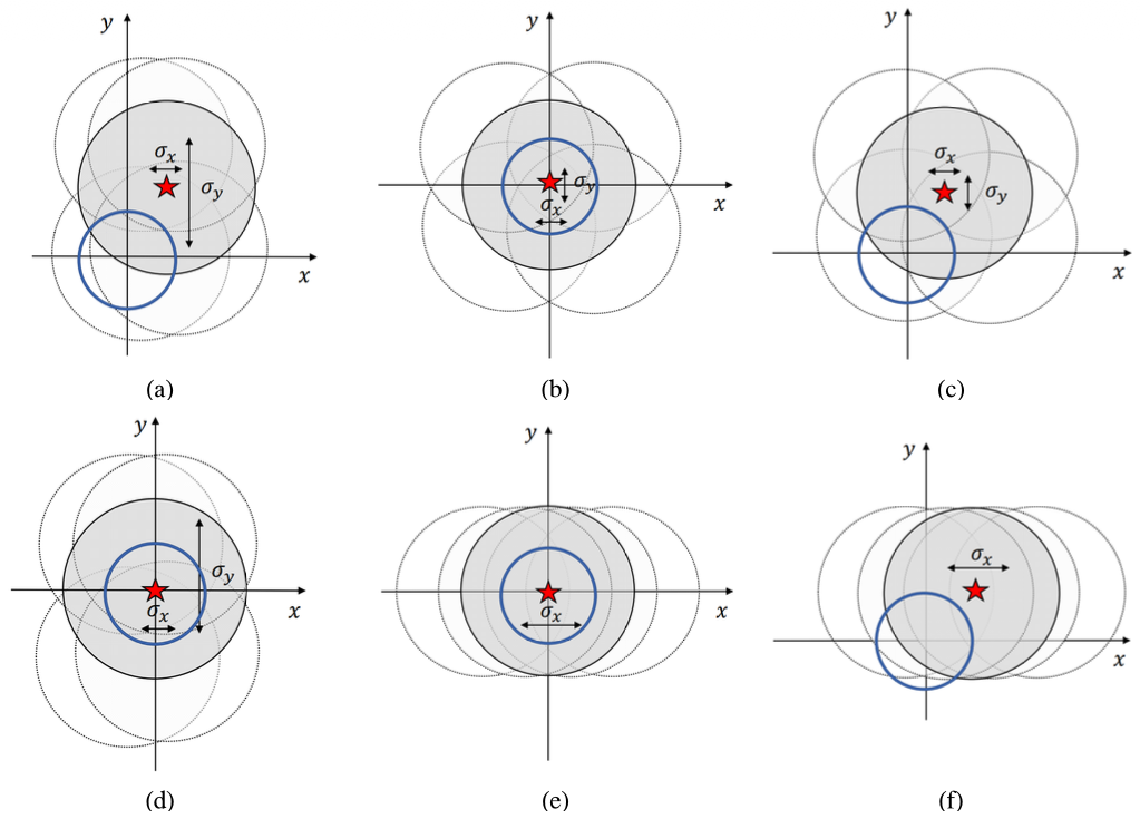

1) Beckmann Distribution

The Beckmann distribution is the generalization of all other models as r_x and r_y follow two independent Gaussian distributions,

In this paper, we focus on the most complicated but general case where μ_x ≠ μ_y and σ_x ≠ σ_y. The beam footprint and PDF in the Beckmann distribution are shown in Fig. 2(a) and (4) [8,Eq.(3)], respectively.

2) Rayleigh Distribution

The Rayleigh distribution is one of the most widely known distribution and the simplest case. The components of pointing-error radial displacement follow the same Gaussian distribution such as

For the Rayleigh and Rician models, we assume isotropic jitter, i.e., jitters in the x- and y-axes are identical (σ_x = σ_y = σ). This is consistent with widely used models in the literature^[8] and simplifies the statistical expressions. The beam footprint and PDF for the Rayleigh distribution are shown in Fig. 2(b) and (5) [8,Eq.(7)], respectively.

3) Rician Distribution

The Rician distribution is similar to the Rayleigh distribution except that the boresight is non-zero. Hence, the radial displacement follows two distinct Gaussian distributions such as

The beam footprint and PDF for the Rician distribution are shown in Fig.2(c) and (6)[8,Eq.(10)], respectively. In (6), [TeX:] $$I_0(\cdot)$$ is the modified Bessel function of the first kind of order zero.

4) Hoyt Distribution

The Hoyt distribution is also similar to Rayleigh distribution, but the jitters in the x-axis and y-axis differ. Thus, the radial displacement is expressed as

The beam footprint and PDF for the Hoyt distribution are shown in Fig. 2(d) and (7) [8, Eq. (13)], respectively.

5) Zero-mean single-sided Gaussian Distribution

In this scenario, the jitter occurs in only one direction, either parallel or perpendicular to the receiver plane as depicted in Fig. 2(e). In this paper, we only consider the jitter along the x -axis. The PDF of this distribution can be derived through a simple random variable transformation using (2) and [8, Eq.(16)] as (8).

6) Non-zero mean single-sided Gaussian Distribution

This distribution corresponds to the non-zero boresight case for the Zero-mean single-sided Gaussian distribution. Here, we consider the case that μ_x = μ_y and the jitter along the x-axis. The beam footprint and PDF of the distribution are shown in Fig. 2(f) and (9), respectively. In (9), [TeX:] $$I_{-\frac{1}{2}}(\cdot)$$ is the modified Bessel function of the first kind of order [TeX:] $$-\frac{1}{2}$$. The PDF can be derived via a simple random variabl transformation using (2) and [9, Eq.(7)].

2.3 Relationship between Pointing-Error Radial Displacement and Pointing Error

In this paper, we distinguish between two similar looking terms: the pointing-error radial displacement and the pointing error. The former refers to the radial displacement (in meters) of the beam within the receiver aperture caused by pointing error (in radians), whereas the latter denotes the pointing error at the transmitter side. The relationship between the pointing-error radial displacement and the pointing error is illustrated in Fig. 3. Here, r is the pointing-error radial displacement, dis the ISL distance between the source satellite and the destination satellite, and θ_T is the pointing error. By applying basic trigonometry, the relationship between these elements can be expressed as [TeX:] $$r=d \tan \left(\theta_T\right)$$. In this paper, we use the approximation [TeX:] $$\tan \left(\theta_T\right) \approx \theta_T$$, since the θ_T is extremely small given that the ISL distance ranges from several hundred to several thousand kilometers. This approximation yields the final relationship between the pointing-error radial displacement and the pointing error as

Fig. 3.

2.4 Pointing Error Statistical Model

By applying a simple random variable transformation between r and q T as in (13), given by [TeX:] $$f_{\theta_T}\left(\theta_T\right)=f_r(r) \cdot\left|\frac{\partial r}{\partial \theta_T}\right|$$, the PDFs of the pointing error can be derived from Table 1, as summarized in Table 2. Since the PDFs of the pointing error involve the ISL distance d, the distribution of the pointing error varies with the link distance.

2.5 Inter-Satellite Link Distance

To determine realistic ISL distances, we refer to SpaceX’s Starlink constellation as analyzed in[5]. In the proposed modification scenario for phase Ⅰ, total 1,584 satellites are deployed in 24 orbital planes with an inclination of 53° at the altitude of 550 km. This scenario is illustrated in Fig. 4. Here, r is the Earth’s radius, which is 6,378 km; h_s is the satellite altitude, which is 550 km; h_t is the minimum altitude above which atmospheric effects are negligible, set to 22km^[10]; and θ is the radial interval between adjacent satellites in the same orbital plane, which can be calculated as

Here, we determine the minimum and the maximum ISL distances between two satellites in the same orbital plane. The minimum ISL distance can be obtained using basic trigonometry and a degree-to-radian conversion, yielding [TeX:] $$d_{\min }=2 \times\left(r+h_s\right) \times \sin (\theta / 2)=659 \mathrm{~km}$$. The maximum link distance can also be calculated by using basicg eometry, yielding

[TeX:] $$d_{\max }=2 \times \sqrt{\left(r+h_s\right)^2-\left(r+h_t\right)^2}=5,305.53 \mathrm{~km}$$.

For analytical tractability, this study focuses on intra-orbital plane ISLs, where both satellites reside in the same orbital plane. Extension to more realistic scenarios, including inter-orbital plane ISLs with varying inclinations, will be considered in future work.

Ⅲ. Link Budget Analysis

3.1 Link Budget

In space-based FSO communication, where atmospheric attenuation is negligible, the relationship between the transmitted power P_T and the received power P_R is expressed as

where P_T and P_R are expressed in dBm, and all other terms are in dB. Here, η_T is the transmitter optical efficiency, η_R is the receiver optical efficiency, G_T is the transmitter gain, G_R is the receiver gain, L_T is the transmitter pointing loss, L_R is the receiver pointing loss, and L_PS is the free-space path loss between satellites^[12]. The transmitter gain is expressed as

where Θ_T is the full transmitting divergence angle. The receiver gain is expressed as

where D_Ris the receiver aperture diameter and λ is the laser wavelength. The transmitter pointing loss is expressed as

where θ_T is the transmitter pointing error. The receiver pointing loss is expressed as

where θ_R is the receiver pointing error. The transmitter and receiver pointing losses range between 0 and 1. As either of the pointing error increases, the corresponding pointing loss approaches zero, indicating a significant signal degradation. The free-space path loss is expressed as

where d is the ISL distance. For simplicity, we assume θ_R=0 in this paper, which leads to L_R=1, as the analysis focuses on the transmitter pointing error with respect to the receiver. Applying this assumption to (21) yields the simplified link budget equation as

3.2 Transmit Power Calculation

Since the transmitter pointing loss L_T is a function of the transmitter pointing error θ_T ,the expected value of L_T can be expressed as

Closed form expressions of [TeX:] $$E\left[L_T\right]$$ are derived and listed in Table 3. Here, note that unlike the other pointing error models considered in this study, the Beckmann model does not admit a closed-form expression for the expected pointing loss [TeX:] $$E\left[L_T\right]$$. This is due to the presence of a non-separable, anisotropic Gaussian kernel over angular variables, compounded with a θ_T-dependent exponential term, making the double integral analytically intractable.

Applying (34) into (33) yields the link budget equation as

Ⅳ. Numerical Results

4.1 Simulation Settings

In this section, we present the numerical evaluation of the required transmit power that meets the receiver sensitivity of -35.5 dBm under the comprehensive six different pointing error models presented in Table 2. The parameter settings are provided in Table 4 and 5. The performance is assessed for five ISL distances: d_min = 659km, 2,000 km, 3,000 km, 4,000 km, and d_max = 5,305.53 km. Both the closed-form analytical expressions and the MonteCarlo simulation results are illustrated in Fig. 5, and the numerical values are provided in Table 6. All MonteCarlo simulations use 10⁶ samples.

Fig. 5.

Transmit power versus jitter level for comprehensive six pointing error models: (a) Beckmann distribution, (b) Rayleigh distribution, (c) Rician distribution, (d) Hoyt distribution, (e) Zero-mean single-sided Gaussian distribution, (f) Non-zero mean single-sided Gaussian distribution. The curves are color-coded by link distance in ascending order: blue (659 km), purple (2,000 km), green (3,000 km), orange (4,000 km), and red (5,305.53 km).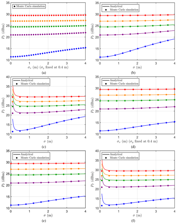

The jitter varies from 0.01 m to 4 m for most models. However, for the Rician and Non-zero mean single-sided Gaussian models, the simulation range starts at 0.1m instead of 0.01m. In these two models, P_T increases sharply as the jitter approaches zero. This is due to the non-zero boresight offset, which causes the beam to focus in a fixed, misaligned direction when jitter approaches zero. As a result, most of the beam misses the small receiver telescope, leading to near-zero received power and thus a divergent P_T. While MonteCarlo simulations smooth out this effect due to averaging, the closed-form expression captures the deterministic misalignment explicitly.

In the Beckmann and Hoyt models, jitter exists in both the x- and y-axes. To isolate the impact of horizontal jitter and enable a controlled 2D performance evaluation, the vertical jiter σ_y is fixed at 0.4m, while σ_x varies from 0.01m to 4m.

4.2 Model-by-Model Comparison

1) Rayleigh and Rician Models

The Rayleigh and Rician models exhibit very similar trends in required transmit power P_T across the entire jitter range, particularly at shorter ISL distances where P_T increases by approximately 7.96 dB and 7.93 dB, respectively, at 659km. While this similarity is expected at large σ due to the diminishing influence of the fixed boresight in the Rician model, it also appears at small σ, which may seem counterintuitive. This is because the Rician factor [TeX:] $$K=\frac{\mu_x^2+\mu_y^2}{2 \sigma^2}$$ remains modest (e.g., [TeX:] $$K \approx 0.77$$ when μ_x=0.03m, μ_y=0.12m, and σ=0.1m), making the effect of the boresight relatively weak even in the low-jitter regime. Additionally, since the Rician simulations start at σ=0.1m, the regime where deterministic misalignment dominates is excluded, further contributing to the observed similarity with the Rayleigh case.

2) Beckmann and Hoyt Models

The Beckmann and Hoyt models exhibit relatively stable transmit power performance across the entire jitter range. At 659km, the required transmit power increases by only 3.97dB under the Beckmann model and shows nearly identical behavior under the Hoyt model. Even at higher distances such as 5,305.53km, the increase remains below 0.2 dB. This stability stems from the directional configuration of the jitter: while the horizontal jitter component σ_x varies from 0.01m to 4m, the vertical jitter σ_y is fixed at 0.4 m. Because the overall misalignment is governed by the combined radial displacement, the contribution of σ_x becomes relatively less significant when σ_y is already large. As a result, additional jitter in the horizontal direction causes only marginal degradation in pointing accuracy. This anisotropic behavior underscores the importance of dominant-axis jitter in link performance and highlight show a single direction can saturate the system's sensitivity to further misalignment.

3) Zero-mean single-sided Gaussian and Non-zero mean single-sided Gaussian Models

These models represent single-axis jitter distributions—without and with a deterministic boresight offset, respectively. Despite their structural differences, both exhibit nearly identical transmit power trends. At 659km, the required transmit power increases by approximately 3.98dB and 3.97dB for the zero-mean and non-zero mean cases, respectively, across the full jitter range. At 5,305.53km, the difference becomes negligible, with both models showing a variation of less than 0.2dB. These results indicate that when jitter is confined to a single direction, even large variations in its magnitude lead to only modest changes in transmit power. This suggests that it is not just the presence of jitter, but how broadly it spreads across spatial dimensions, that determines its impact on link performance.

4.3 General Observations and Summary

Across all models, shorter ISLs exhibit greater sensitivity to jitter due to their narrower beam footprints. The required P_T consistently stays below 30 dBm under all conditions, satisfying the transmit power constraints of Mynaric's laser communication terminal^[12]. Furthermore, the closed-form analytical results align closely with the Monte Carlo simulations, confirming the accuracy of the derived expressions.

Ⅴ. Conclusion

In this work, we presented comprehensive six statistical models of pointing error affecting FSO systems in ISLs, and determined realistic ISL distances based on SpaceX’s Starlink constellation. We then analyzed the link budget for each pointing error model under five different ISL distances, with respect to jitter. Finally, we compared the closed-form analytical expressions with rigorous Monte Carlo simulations using 10⁶ samples for each setting to verify the accuracy and applicability of the derived formulations.

The simulation results confirm that the required transmit power P_Tremains within 30 dBm under all considered models and distance scenarios. This satisfies the practical constraint of 1 W optical transmit power used in Mynaric's commercial laser communication terminal, validating the feasibility of robust FSO-based ISLs even under statistically significant pointing uncertainties.

Overall, this study offers a unified and extensible modeling framework to evaluate pointing error impact on ISL link budgets. The findings reinforce the importance of statistical error modeling and show that closed-form expressions, when used carefully with respect to their assumptions, can provide valuable design guidance.

In future work, this framework may be extended by incorporating time-varying jitter processes, satellite body dynamics, and adaptive power control strategies. Further exploration of coding/modulation adaptation and acquisition/tracking mechanisms under the derived statistical distributions would also provide valuable insights toward the development of robust next-generation optical ISLs.