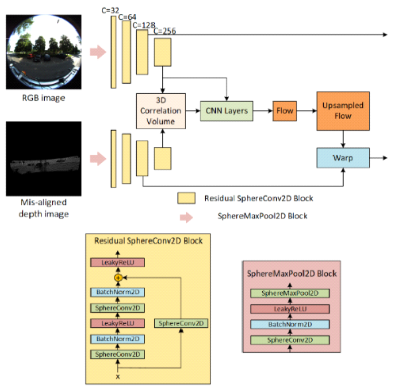
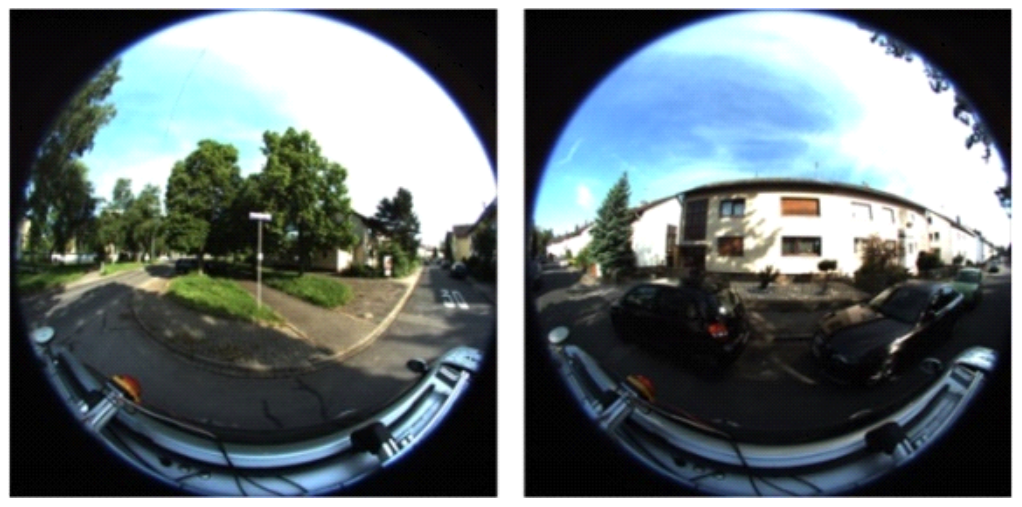
Deep Learning-Based Lightweight LiDAR and Fisheye Camera Online Extrinsic Calibration

Ⅰ . Introduction

Autonomous driving technology, an emerging field that enables vehicles or robots to navigate and operate without human intervention, can potentially revolu- tionize transportation and has therefore attracted much attention from both academicians and industrial researchers. Many state-of-the-art methods achieve autonomous functionality through advanced tech- nologies, seeking more localized and efficient sensor solutions than satellite-based systems such as Global Positioning Systems and Global Navigation Satellite Systems, which are primarily limited by high latency. The combination of camera and Light Detection and Ranging (LiDAR) data is considered as a standout ap- proach for autonomous driving systems^[1].

Cameras capture high-resolution, color-rich im- agery of the surrounding environment, enabling the detection and recognition of objects, textures, and oth- er visual details with remarkable clarity. The standard pinhole camera is widely used because it is both sim- ple and effective, but its field-of-view (FoV) is limited to 80°. An ultrawide FoV (180°) is provided by fish- eye cameras, which can capture substantially more da- ta and features in a single image than pinhole cam- eras^[2].

However, as camera sensors cannot measure dis- tances directly, they cannot adequately capture the depth information. The limited depth perception chal- lenges the interpretation of spatial relationships be- tween the vehicle and its surroundings objects.

Unlike traditional cameras, LiDAR sensors provide precise distance measurements. The collected data are represented as a three-dimensional array of points with X, Y, and Z coordinates in a Cartesian system. These arrays, called point clouds, provide a detailed spatial representation of the environment. Accordingly, LiDAR is a critical component in auton- omous driving systems.

Despite these advantages, the high cost and compu- tational intensity of LiDAR devices greatly raises the cost of large-scale deployment. In addition, LiDAR data are inherently sparse and lack red–green–blue (RGB) color information, complicating their inter- pretation and processing^[3].

To avoid these limitations, LiDAR and camera sen- sors data are commonly combined in recent autono- mous driving systems. The integration of cameras and LiDAR can notably enhance the capabilities of both autonomous driving and robotics systems. However, the simultaneous deployment of multiple sensors in- creases the computational complexity of the system. The data generated by these sensors can be highly diverse and complex, requiring sophisticated process- ing to extract meaningful insights.

Traditionally, feature extraction and decision-mak- ing tasks based on fusion sensor data have been per- formed by algorithms such as Iterative Closest Point^[4], RANSAC^[5], and K-Means^{[ 6]}. Although these methods perform effectively in structured or static en- vironments, they are often less successful under dy- namic driving conditions.

In recent years, deep learning has become a focal point of both research and practical applications. Researchers in the autonomous driving and robotics fields have explored ways of integrating deep learning techniques into their workflows. Given high-quality and normally distributed data, a well-designed deep learning methods leverage neural networks to adapt to variations in sensor viewpoints, lighting conditions, and environmental dynamics, making them effective for extrinsic LiDAR-camera calibration in complex and unstructured environments.

The present study proposes a deep learning-based online extrinsic calibration method that fuses the data of LiDAR and fisheye camera sensors. Leveraging the complementary strengths of the two sensors, the meth- od aims to enhance the capabilities of autonomous driving and robotic systems. Whereas LiDAR pro- vides precise distance measurements between the sen- sor (or vehicle) and surrounding objects, the fisheye camera captures a comprehensive 180° RGB repre- sentation of the environment.

Ⅱ. Related Research

Both the intrinsic and extrinsic parameters of each sensor in the data-fusion system must be calibrated to ensure accurate data integration. In this work, we assume that the intrinsic parameters of the fisheye camera and LiDAR provided in the dataset have been calibrated by the manufacturer, as we follow similar studies^[7,8]. Therefore, only extrinsic calibration is con- sidered here. However, for real-environment applica- tion, we acknowledge that even minor residual errors in intrinsic calibration can affect the extrinsic calibra- tion accuracy.

The existing LiDAR-Camera calibration methods can be broadly categorized into target-based, target- less, and learning-based methods. These three catego- ries are summarized below.

2.1 Target-based Methods

For accurate calibration, target-based methods fre- quently establish the correspondence between two-di- mensional (2D) camera images and three-dimensional (3D) LiDAR points of specially designed objects.

Checkerboards have been extensively utilized in target-based extrinsic calibration studies. For instance, Geiger et al.^[9] calibrated LiDAR and cameras by de- tecting the corners of checkerboard patterns and esti- mating the transformation matrix between the two sensors. Similarly, Wang et al.^[10] proposed an online extrinsic calibration method employing a checker- board for 3D LiDAR and panoramic cameras.

2.2 Targetless methods

In real-world autonomous driving and robotics sce- narios, where ideal calibration targets such as checker- boards are often unavailable, researchers have devel- oped various targetless methods.

For instance, Song et al.^[11] proposed the Galibr method, which performs extrinsic LiDAR and camera calibration through ground plane features. Borer et al.^[12] calibrated LiDAR and its fisheye camera using a continuous online extrinsic calibration approach based on a mutual-information matching method.

2.3 Learning-based Methods

Deep learning has been widely adopted in extrinsic calibration scenarios. Lv et al.^[7] introduced LCCNet, a neural network model for LiDAR and camera self-calibration, which leverages a cost volume layer to facilitate feature matching between RGB image fea- tures and depth map features. Wang et al.^[8] proposed Multiresolution LiDAR-Camera Calibration Network (MRCNet), an end-to-end neural network that inputs the RGB image and the depth image generated from the LiDAR point cloud and predicts the trans- formation matrix for extrinsic calibration. Their net- work adopts a geometric feature-constraint module and performs multiresolution feature extraction and feature matching. Zhu et al.^[13] proposed CalibDepth, which also relies on RGB and depth images. The depth image in CalibDepth provides a unified repre- sentation, bridging the gap between the RGB image data and the point cloud inputs. CalibDepth also in- corporates long short-term memory for autoregressive generation of the calibration actions at each step.

The abovementioned studies highlight a notable lack of research on extrinsic calibration between LiDAR and fisheye cameras, particularly in learn- ing-based approaches. In this study, we design an end-to-end, deep learning-based online extrinsic cali- bration method for LiDAR and fisheye cameras.

Ⅲ . Proposed Methods

The proposed model integrates a residual spherical convolution layer for feature extraction from fisheye images with an optical flow based on the depth map.

3.1 Problem Formulation

Given a multimodal input composed of RGB im- ages and a LiDAR point cloud, online extrinsic cali- bration obtains a transformation matrix T consisting of a 3 × 3 rotation matrix and 1 × 3 translation vector. During the learning process, a random transformation T_rand is applied to matrix T , obtaining an initial matrix T_init . T_init is then applied to the point cloud to obtain a mis-calibrated depth image. Projection matrix fish- eye-depth images were generated as described in [14]. The objective of the proposed model is to estimate the extrinsic calibration matrix T_rand , denoted as T_pred , based on the RGB image and the point cloud using the mis-calibrated depth image.

Fig. 1.

Architecture of the proposed model.

3.2 Network Architecture

Our proposed model is divided into three main components: feature extraction, feature matching, and a regression layer. This subsection describes each component in detail.

3.2.1 Feature Extraction

Feature extraction by the proposed model occurs through two parallel branches, one for the fisheye RGB image, the other for the mis-calibrated depth map. To effectively handle the spherical images gen- erated by the fisheye camera, we introduce a residual spherical feature-extraction technique to both branches. This approach builds upon a modified spherical convolution of SphereNet^[15], adapting it to a residual framework to capture the semantic features in both the original and refined inputs, ultimately en- hancing the quality of the extracted features.

The spherical convolution of SphereNet lifts the kernel of a 3 × 3 convolution layer into spherical space. The kernel shape is defined in spherical space with [TeX:] $$\begin{equation} j, k \in\{-1,0,1\} \end{equation}$$ and step sizes of [TeX:] $$\begin{equation} \Delta_\theta \end{equation}$$ and [TeX:] $$\begin{equation} \Delta_\phi \end{equation}$$.

The kernel sampling s is defined as

where θ measures the inclination from the positive z-axis downward (ranging from 0° at the north pole to 180° at the south pole), while φ measures the rota- tion around the z-axis in the xy-plane, increasing counterclockwise from a reference direction (typically the positive x-axis).

3.2.2 Feature Matching

The feature matching layer is inspired by MRCNet^[8], which creates a 3D correlation volume representing the spatial correlation between the fea- tures extracted from RGB image and LiDAR depth map. The 3D correlation volume is defined as

where x_rgb and x_lidar denote a feature in the RGB image and depth map respectively, D represents the search region where feature correspondences are computed, while p_i and p_j denote pixel locations in the RGB im- age and the depth map. The optical flow between the two feature sets is then estimated from the 3D correla- tion volume within a learning-based layer, comprising a regular convolutional layer that outputs a channel of size two representing the horizontal and vertical flow vectors. In this study, the depth map was taken as the “target” of the optical flow.

3.2.3 Regression Layer

The regression layer inputs the features xwith the finest resolution and processes them through multiple convolutional layers, followed by an average pooling layer that condenses the features. The pooled features are flattened and then passed into a fully connected layer along with an activation function LeakyReLU

where α is a small constant. Afterwards, the feature xis passed into a dropout layer. The process can be represented mathematically as

where Bis batch size. This operation reshapes pooled feature x from B × C × 1 × 1 to a vector of size B × C.

The reshaped feature is passed into two prediction branches: one for rotation in quaternion q format and the other for predicting the X , Y , and Zcomponents of the translation vector t . Subsequently, the predicted quaternion is normalized as below

where [TeX:] $$\begin{equation} \epsilon(\epsilon=1 e-10) \end{equation}$$ is a small constant added for numerical stability. The output T_pred is a normalized quaternion vector and a translation vector, which can be represented as

where [TeX:] $$\begin{equation} q_{\text {norm }} \in \mathbb{R}^4 \end{equation}$$ is the normalized quaternion vector and [TeX:] $$\begin{equation} t \in \mathbb{R}^3 \end{equation}$$ is the translation vector.

3.3 Loss Functions

In this study, the loss functions of both quaternion and translation predictions in T_pred are expressed in terms of the Euclidean distance. The Euclidean-dis- tance loss functions of translation and rotation are re- spectively defined as

where [TeX:] $$\begin{equation} \mathcal{L}_t^l \end{equation}$$ is translation loss, [TeX:] $$\begin{equation} t^l \end{equation}$$ is predicted translation and [TeX:] $$\begin{equation} t_{gt}^l \end{equation}$$ is ground truth translation. Similarly, [TeX:] $$\begin{equation} \mathcal{L} r^l \end{equation}$$ is rotational loss, [TeX:] $$\begin{equation} q^l \end{equation}$$ is predicted quaternion and [TeX:] $$\begin{equation} q_{gt}^l \end{equation}$$ is ground truth quaternion.

3.4 bration Inference

Similarly to [7] and [8], the designed network does not directly predict the extrinsic calibration matrix. As the generated depth image is based on the mis-calibra- tion matrix T_rand , the predicted matrix will express the deviations from the initial parameters. To obtain the extrinsic calibration matrix, the quaternion q in T_pred is first converted into a standard 3 × 3 rotation matrix, which can be represented as

where Ris 3 × 3 rotation matrix and w , x , y , zis the element in quaternion vector q = ( w , x , y , z ). Finally, the T matrix is computed as follows

Fig. 2.

Examples of fisheye images from the KITTI-360 dataset

where T_pred is predicted transformation matrix misalignment and T_init is the matrix multiplication of transformation matrix misalignment T_rand and ground truth extrinsic parameters T .

Several learning-based methods for extrinsic cali- bration [7] and [8] employ an iterative inference ap- proach, which progressively refines the calibration through multiple networks across different ranges. In contrast, this study only employs single model ap- proach similar to that in [16].

Ⅳ . Experiment

4.1 Dataset

The experiment was conducted on the Karlsruhe Institute of Technology and Toyota Technological Institute (KITTI)-360 dataset, which comprises eight sequences taken by four cameras, two utilizing fisheye lenses. The fisheye cameras of the KITTI-360 dataset use the model of Mei and Rives^[15] as the projection model.

The present experiment was conducted on fisheye images from camera 2 (76,251 images in total). We also used the Velodyne HDL-64E LiDAR point cloud data provided in the KITTI-360 dataset for depth map generation. The fisheye images and LiDAR have been already synchronized in the dataset. All sequences ex- cept sequence 00 were used for training; the remaining was reserved for testing and validation.

As mentioned in Section III, the point cloud data were mis-calibrated using T_rand and projected onto the 2D fisheye image. The initial translation and rotation misalignments were 0.5 meter and 5.0°, respectively. Following^[7], the RGB images were augmented with color jittering alone.

4.2 Training Details

The proposed deep learning model was im- plemented using the PyTorch library and trained on an NVIDIA RTX 3090Ti GPU (24GB), paired with an Intel Xeon 4215R CPU and 32GB of ran- dom-access memory (RAM). The model includes ap- proximately 8M parameters. Training was performed with a batch size of 16 over 75 epochs. The initial learning rate was set to 1e−4 and was reduced by a factor of 0.3 whenever the validation performance stagnated for 10 consecutive evaluations.

4.3 Results and Discussion

In this experiment, our approach operates within a maximum initial misalignment of 5.0° in rotation and 0.5 meter in translation. The translation error E_t , defining the Euclidean distance between the predicted translation t_pred and ground truth translation t_gt , is mathematically expressed as

where t_gt and t_pred are ground truth and predicted trans- lation respectively. Meanwhile, E_r is calculated using the quaternion distance formula. The quaternion dis- tance is computed as

where q_gt is the ground truth quaternion, q_pred is pre- dicted quaternion and [TeX:] $$\begin{equation} t_w, t_x, t_y, t_z \end{equation}$$ are the Hamilton products of q_gt and q_pred . In addition, we provide the absolute error on each translation axis (X , Y , Z ) and in each rotational angle (roll,pitch,yaw ). The roll, pitch, yaw are defined as

where R_pred is the 3 × 3 predicted rotation matrix con- verted from predicted quaternion q_pred .

Given the limited references of learning-based LiDAR and fisheye camera calibration, particularly on the KITTI-360 dataset, we also benchmarked our model against other models trained on regular pinhole camera images from the KITTI Odometry dataset us- ing similar training methods. The KITTI Odometry consists of 22 sequences with 43,552 frames in total. All comparisons were performed at initial translation and rotation misalignments of 0.5 meter and 5.0°, re- spectively, and all reported metrics are the means of all sequences. The comparison results are presented in Table 2.

The proposed method outperforms the approach of Borer et al.^[12] in terms of rotation accuracy, but as Borer et al. did not report the translation performance, the translation misalignment in their method is not di- rectly comparable with ours. Furthermore, Borer et al.’s method is not a deep learning-based method. Compared to KITTI Odometry dataset methods, our model achieves misalignment prediction performance comparable to those methods within a similar max- imum misalignment range.

We also evaluate our method alongside other deep learning-based approaches by comparing model re- source utilization during inference such as parameter count, inference time, GPU memory usage, and stor- age capacity. For iterative methods, since they have multiple trained models, we selected a single model with an initial misalignment similar to our approach. The results were replicated in a resource-constrained setup featuring an NVIDIA RTX 3060 (8GB), an Intel i7-12700 (12th Gen) processor, and 16GB of RAM. The operating system is Ubuntu 20.04. The number of workers used for the GPU is 0 and the batch size is set to 1. The findings are summarized in Table 3. This evaluation highlights the model’s efficiency un- der limited computational resources, reinforcing its practicality for real-world deployment.

As seen in Table 3, our proposed model has a slightly slower inference time compared to MRCNet^[8]. However, in other aspects, such as param- eter count, GPU memory usage, and storage require- ments, our model is significantly more efficient. This highlights the lightweight property of our model and its suitability for real-time inference.

Fig. 3.

Estimated extrinsic calibration using the proposed deep learning model. From left to right, each row shows the initial misalignment, ground truth, and calibrated image results.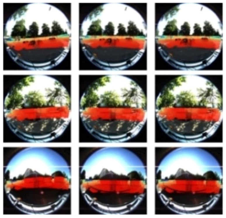

The extrinsic calibration results are visualized in Fig. 3. As shown in the image, the LiDAR point cloud projection closely resembles the ground truth, indicat- ing that both the LiDAR and fisheye camera are cali- brated with minimal misalignment.

Ⅴ . Conclusion

We proposed a deep learning-based method for ex- trinsic calibration between LiDAR and fisheye cameras. The model introduces a feature-extraction approach using residual SphereConv2D, an enhance- ment of SphereConv2D from SphereNet. In addition, it incorporates optical flow with a depth image as the flow reference. This lightweight model with only 8M parameters is designed for real-time applications.

The proposed method calibrates the extrinsic pa- rameters under initial misalignments of up to 0.5 me- ter in translation and 5.0° in rotation. It achieves mean translation errors of 1.375, 0.753, and 1.208 cm along the X , Y , and Zaxes, respectively, and mean rotation errors of 0.171°, 0.150°, and 0.089° in the roll, pitch, and yaw directions, respectively.