IndexFiguresTables |
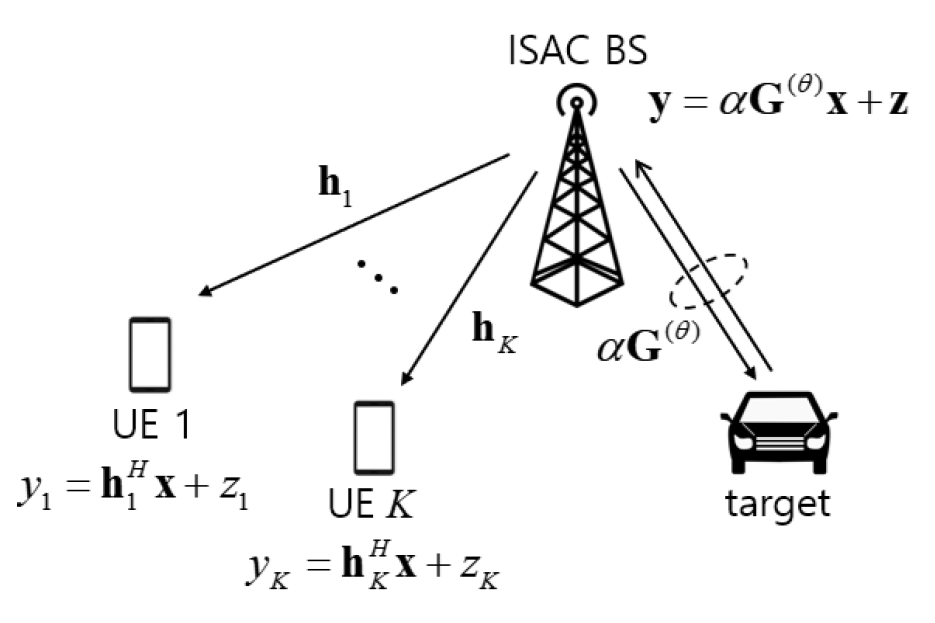
Seok-Hwan Park♦°Fractional Programming for Multi-User ISAC Beamforming Design: A Bayesian CRB PerspectiveAbstract: Integrated sensing and communication (ISAC) is a promising paradigm for sixth-generation (6G) wireless networks, enabling spectrum-efficient coexistence of sensing and communication functionalities. This paper investigates ISAC beamforming optimization for a multi-user system, where a base station (BS) serves multiple communication user equipments (C-UEs) while sensing a target of interest. We adopt the Bayesian Cramer-Rao bound (BCRB) as the sensing performance metric, which is a expected value of CRB with respect to the target prior distribution. An optimization problem is formulated to minimize the BCRB while ensuring that C-UEs’ signal-to-interference-plus-noise ratios (SINRs) exceed predefined thresholds. To address the inherent non-convexity, we employ the fractional programming (FP), leading to a structured reformulation that enables efficient optimization. An alternating optimization (AO) algorithm is developed to iteratively update the primary beamforming and auxiliary variables, ensuring monotonic decrease of BCRB values. Numerical results validate the effectiveness of the proposed FP approach, demonstrating improved sensing accuracy while maintaining reliable communication performance. Keywords: Integrated sensing and communication , multi-user , beamforming , fractional programming , Bayesian CRB Ⅰ. IntroductionIntegrated sensing and communication (ISAC) is envisioned as a key enabler for sixth generation (6G) wireless systems, where sensing and communication share a common platform and spectrum resource[1]. ISAC is expected to significantly reduce system costs and improve spectral efficiency. To effectively balance sensing and communication performance, careful beamforming design for ISAC transmission and reception is essential[2-7]. However, optimizing ISAC beamforming is challenging due to the presence of two distinct and sometimes conflicting objectives. Extensive research has been conducted on ISAC beamforming optimization, with studies categorized basewd on the adopted sensing metric. In [2] and [3], the Cramer-Rao bound (CRB) on the target parameter was used as the sensing metric. However, since CRB depends on the target parameter, it is applicable only when beam sweeping is performed with a tentative estimate available. An alternative metric is the Bayesian CRB (BCRB)[4-6], also known as the posterior CRB[7], which represents the expected value of CRB with respect to the prior distribution of the target parameter. This allows BCRB to be evaluated and used for ISAC beamforming design utilizing only the target prior distribution. Beamforming design based on the BCRB criterion was studied in [5] for a multi-user ISAC system, in which a base station (BS) serves multiple communication user equipements (C-UEs) while sensing a target via received echo signals. A key contribution of [5] was demonstrating the opportunity to leverage the well-established uplink-downlink duality of communication channels[8] for ISAC beamforming design. However, the optimization algorithm for obtaining the optimal ISAC beamforming vectors was not explicitly derived in [5]. In this work, we address ISAC beamforming optimization for a multi-user ISAC system using the fractional programming (FP) approach[9]. Specifically, we formulate a problem that minimizes the BCRB metric while ensuring that the signal-to-interference- pluse-noise ratios (SINRs) at C-UEs exceed a given threshold level. We show that the BCRB metric, which involves a 3-by-3 matrix inversion, can be simplified to a closed-form expression by utilizing the independence between the target parameter and nuisance parameters. To tackle the non-convexity of the resulting problem, we employ the matrix quadratic transform[9, Thm. 1], leading to a joint optimization over primary beamforming and auxiliary variables. We then develop an alternating optimization (AO) algorithm that iteratively updates these variables, ensuring monotonically decreasing BCRB values. Numerical results validate the effectiveness of the proposed ISAC beamforming design. Ⅱ. System ModelAs illustrated in Fig. 1, we consider a multi-user ISAC system where a BS, equipped with [TeX:] $$N_T$$ transmit antennas, serves K single-antenna C-UEs while simultaneously sensing a target of interest using [TeX:] $$N_R$$ receive antennas. The set of communication users’ indices is denoted as [TeX:] $$[K]=\{1,2, \ldots, K\} .$$ 2.1. Communication Channel ModelAssuming a flat-fading channel model, the received signal at the k–th C-UE is given by
where [TeX:] $$h_k \in C^{N_T \times 1}$$ is the channel response vector between the BS and C-UE k, [TeX:] $$x \in C^{N_T \times 1}$$ is the transmitted signal vector from the BS, and [TeX:] $$z_k \sim C N\left(0, \sigma_C^2\right)$$ is additive noise with variance [TeX:] $$\sigma_C^2.$$ The transmitted signal x is subject to the power constraint:
where P denotes the power budget. We define the transmit signal-to-noise ratio (SNR) of the communication channel [TeX:] $$S N R_C$$ as the ratio between the transmit power budget P and the noise power [TeX:] $$E\left[\left|z_k\right|^2\right]=\sigma_C^2,$$ i.e.,
2.2 Sensing Channel ModelThe transmitted signal vector x propagates through the wireless environment and is reflected by the target of interest before arriving at the receive antennas of the BS. The received signal vector [TeX:] $$y \in C^{N_R \times 1}$$ is modeled as
where [TeX:] $$\alpha G^{(\theta)} \in C^{N_R \times N_T}$$ represents the target response channel matrix, and [TeX:] $$z \sim C N\left(0, \sigma_S^2 I\right)$$ denotes the additive noise vector. The complex reflection coefficient [TeX:] $$\alpha \sim C N\left(0, \sigma_\alpha^2\right)$$ here captures the effect of the radar cross-section (RCS), while the remaining factor [TeX:] $$G^{(\theta)} \in C^{N_R \times N_T}$$ of the target response channel depends on the angle-of-arrival (AoA) [TeX:] $$\theta \in[-\pi, \pi]$$ as
where [TeX:] $$a_R(\cdot) \in C^{N_R \times 1} \text { and } a_T(\cdot) \in C^{N_T \times 1}$$ are the receive and transmit steering vectors given by
[TeX:] $$a_X(\theta)=\frac{1}{\sqrt{N_X}}\left[1, e^{j \pi 1 \sin (\theta)}, \cdots, e^{j \pi\left(N_X-1\right) \sin (\theta)}\right],$$ for [TeX:] $$X \in\{T, R\}$$ under the assumption of uniform linear arrays (ULAs). Similar to (3), the transmit SNR of the sensing channel [TeX:] $$S N R_S$$ is defined as the ratio between the transmit power budget P and the noise power of each receive antenna [TeX:] $$E\left[\|z\|^2\right] / N_R=\sigma_S^2,$$ i.e.,
It is worth noting that, to highlight the core idea of applying FP to ISAC beamforming design, we focus on a simplified scenario without interference from potential clutters or uplink transmissions in the echo signal y. Extending the design to more practical scenarios involving such interference is left for future work. We define a vector [TeX:] $$\eta=\left[\theta, \alpha_R, \alpha_I\right]^T$$ of unknown parameters, where [TeX:] $$\alpha_R \text { and } \alpha_I$$ denote the real and imaginary components of α. From the observed echo signal y, the BS estimates the AoA θ of the target, while the other unknown parameters [TeX:] $$\alpha_R \text { and } \alpha_I$$ are treated as nuisance parameters. We assume that θ and α are independent, with their marginal distributions [TeX:] $$p(\theta) \text { and } p(\alpha)$$ known a priori. 2.3 ISAC Beamforming ModelWe define the data symbol for C-UE k as [TeX:] $$s_k$$ with [TeX:] $$E\left[\left|s_k\right|^2\right]=1 .$$ The BS applies ISAC beamforming to the data symbols [TeX:] $$\left\{S_k\right\}_{k \in[K]}$$ as
where [TeX:] $$v_k \in C^{N_T \times 1}$$ is the ISAC beamforming vector for [TeX:] $$s_k.$$ As will be detailed in the next subsection, the choice of ISAC beamforming vectors [TeX:] $$v=\left\{v_k\right\}_{k \in[K]}$$ influences not only the communication performance for C-UEs but also the sensing performance. By substituting the beamforming model (6) into the power constraint (2), we obtain
Furthermore, the covariance matrix of the transmitted signal vector x, which determines the sensing performance, is expressed as a function of the ISAC beamformers v as
2.4. ISAC Performance MetricsThe achievable data rate for each C-UE k is determined by the communication SINR defined as
(9)[TeX:] $$\gamma_k(v)=\frac{\left|h_k^H v_k\right|^2}{\sum_{l \in[K] \backslash\{k\}}\left|h_k^H v_l\right|^2+\sigma_C^2} .$$For instance, when ideal Gaussian channel encoding is applied with a sufficiently large blocklength, the maximum achievable data rate [TeX:] $$R_k$$ is given by [TeX:] $$R_k=\log _2\left(1+\gamma_k(v)\right)$$[10]. Thus, when designing the ISAC beamforming vectors v , we enforce that the communication SINR in (9) exceeds a predefined threshold level [TeX:] $$\gamma_{t h} .$$ Regarding the sensing, the BS aims to estimate the AoA θ from the received echo signal y. The mean squared error (MSE) of the AoA θ estimate depends on the choice of estimator and is generally difficult to evaluate. To facilitate the design, we consider the Bayesian Cramer-Rao bound (BCRB)[4-6], which provides a closed-form lower bound on the MSE with the optimal estimator. Specifically, denoting the estimate of [TeX:] $$\theta \text { by } \hat{\theta},$$ the MSE [TeX:] $$E\left[|\theta-\hat{\theta}|^2\right]$$ for any estimator is lower bounded as
where [TeX:] $$J \in C^{3 \times 3}$$ is the Bayesian Fisher information matrix (BFIM), whose (i,j)-th element is given as a function of the covariance matrix Q by
(11)[TeX:] $$[J]_{i, j}=\frac{2 T}{\sigma_S^2} E_\eta\left[\operatorname{Re}\left\{\operatorname{tr}\left(\dot{G}_i^H \dot{G}_j Q\right)\right\}\right]+J_{i, j}^P .$$Here, T denotes the number of samples used for estimation, and we have defined the notations:
(12)[TeX:] $$\begin{aligned} \dot{G}_i & =\frac{\partial}{\partial \eta_i}\left\{\alpha G^{(\theta)}\right\}, \\ J_{i, j}^P & =-E_\eta\left[\frac{\partial^2 \log p(\eta)}{\partial \eta_i \partial \eta_j}\right] . \end{aligned}$$It is important to note that the second term [TeX:] $$J_{i, j}^P$$ in (11) does not depend on the choice of ISAC beamforming vectors v. Ⅲ. Problem Formulation and Optimizationur goal is to optimize the ISAC beamforming vectors v to minimize the BCRB [TeX:] $$\left[J^{-1}\right]_{1,1}$$ in (10) while ensuring that the communication SINRs exceed the given threshold level [TeX:] $$\gamma_{t h} .$$ This leads to the following optimization problem:
(13)[TeX:] $$\begin{array}{ll} \min _v & {\left[J^1\right]_{1,1}} \\ \text { s.t. } & \gamma_k(v) \geq \gamma_{t h}, \forall k \in[K], \\ & \sum_{k \in[K]}\left\|v_k\right\|^2 \leq P . \end{array}$$Solving (13) is challenging due to the non-convexity of the objective function and the communication SINR constraints. Additionally, expressing the objective function [TeX:] $$\left[J^{-1}\right]_{1,1}$$ in a closed-form function of v is difficult, as it involves the inverse of a 3-by-3 matrix J. To address the latter issue first, we derive a closed-form expression of the objective function through the following two theorems. Theor em 1. Let [TeX:] $$\dot{g}_i \in C^{N_R N_T \times 1}$$ denote the vectorization of a matrix [TeX:] $$\dot{G}_i,$$ and consider the singular-value decomposition (SVD) of the matrix [TeX:] $$E_\eta\left[\begin{array}{l} \dot{g}_j \dot{g}_i^H \end{array}\right] \in C^{N_R N_T \times N_R N_T}$$ given by
(14)[TeX:] $$E_\eta\left[\dot{g}_j \dot{g}_i^H\right]=\sum_{r=1}^{R_{j, i}} x_{j, i, r} u_{j, i, r} \hat{u}_{j, i, r}^H$$where [TeX:] $$u_{j, i, r} \in C^{N_R N_T \times 1} \quad \text { and } \quad \hat{u}_{j, i, r} \in C^{N_R N_T \times 1}$$ are the r-th left and right singular vectors, respectively, corresponding to the singular value [TeX:] $$x_{j, i, r}\gt 0 .$$ Then, in the expression of [TeX:] $$[J]_{i, j}$$ in (11), the expectation operator [TeX:] $$E_\eta[\cdot]$$ can be removed, leading to
(15)[TeX:] $$\begin{aligned} {[J]_{i, j} } & =\frac{2 T}{\sigma_S^2} \sum_{r=1}^{R_{j, i}} \operatorname{Re}\left\{x_{j, i, r} \operatorname{tr}\left[\hat{U}_{j, i, r}^H U_{j, i, r} \boldsymbol{Q}\right]\right\} \\ & +J_{i, j}^P . \end{aligned}$$pf) The result in (15) follows directly by applying the same procedure as in the proof of [6, Thm. 1]. Theor em 2. Recalling the assumptions that [TeX:] $$p(\boldsymbol{\eta})=p(\theta) p(\alpha) \quad \text { and } \quad E[\alpha]=0$$ are given in Sec. II.2, we obatin the following equality:
pf) We begin by demonstrating that [TeX:] $$[J]_{2,1}=[J]_{1,2}=0 .$$ The matrix [TeX:] $$E_\eta\left[\dot{g}_2 \dot{g}_1^H\right]$$ can be computed as
(17)[TeX:] $$\begin{aligned} & E_\eta\left[\dot{g}_2 \cdot \dot{g}_1^H\right]=E_\eta\left[\frac{\partial}{\partial \alpha_R}\left\{\alpha g^{(\theta)}\right\}\left(\frac{\partial}{\partial \theta}\left\{\alpha g^{(\theta)}\right\}\right)^H\right] \\ & =E_\eta\left[g^{(\theta)} \alpha^*\left(\frac{\partial}{\partial \theta}\left\{g^{(\theta)}\right\}\right)^H\right] \\ & \stackrel{(a)}{=} \underbrace{E_\alpha\left[\alpha^*\right]}_{=0} E_\theta\left[g^{(\theta)}\left(\frac{\partial}{\partial \theta}\left\{g^{(\theta)}\right\}\right)^H\right] \\ & =0_{N_R N_T \times N_R N_T}, \end{aligned}$$with [TeX:] $$g^{(\theta)} \in C^{N_R N_T \times 1}$$ representing the vectorization of [TeX:] $$G^{(\theta)} .$$ The equality (a) in (17) follows from the independence between [TeX:] $$\theta \text{ and } \alpha .$$ From (17), we obtain [TeX:] $$x_{2,1, r}=0$$ for all [TeX:] $$r \in\left\{1,2, \ldots, R_{2,1}\right\},$$ which leads to
Similarly, following the same procedure, we establish that [TeX:] $$[J]_{3,1}=[J]_{1,3}=0 .$$ Consequently, the BFIM [TeX:] $$[J]_{2,1}=[J]_{1,2}=0 .$$ exhibits a block-diagonal structure of the form:
(19)[TeX:] $$J=\left[\begin{array}{cc} {[J]_{1,1}} & 0_{1 \times 2} \\ 0_{2 \times 1} & {[J]_{2: 3,2: 3}} \end{array}\right] .$$Its inverse can therefore be computed using a block-wise inversion as
(20)[TeX:] $$J^{-1}=\left[\begin{array}{cc} 1 /[J]_{1,1} & 0_{1 \times 2} \\ 0_{2 \times 1} & \left([J]_{2: 3,2: 3}\right)^{-1} \end{array}\right] .$$From (20), it is evident that [TeX:] $$\left[J^{-1}\right]_{1,1}=1 /[J]_{1,1},$$ completing the proof. We note that [TeX:] $$1 /[J]_{1,1}$$ generally serves as a lower bound for [TeX:] $$\left[J^{-1}\right]_{1,1}$$[11]. However, Theorem 2 implies that under our specific problem setting with the assumptions [TeX:] $$p(\boldsymbol{\eta})=p(\theta) p(\alpha) \text { and } E[\alpha]=0,$$ the bound becomes tight. From Theorems 1 and 2, we observe that minimizing [TeX:] $$\left[J^{-1}\right]_{1,1}=1 /[J]_{1,1}$$ is equivalent to maximizing
(21)[TeX:] $$\begin{aligned} & {\left[J^D\right]_{1,1}} \\ & =\frac{2 T}{\sigma_S^2} \sum_{r=1}^{R_{1,1}} \sum_{k \in[K]} \chi_{1,1, r} v_k^H U_{1,1, r}^H U_{1,1, r} v_k . \end{aligned}$$Here, we have removed [TeX:] $$J_{1,1}^P$$ in (21), since it is not dependent on the ISAC beamformers v . Additionally, we have used the identity [TeX:] $$\widehat{U}_{j, i, r}=U_{j, i, r} \text { for } j=i .$$ Therefore, the original optimization problem (13) can be equivalently reformulated as
(22)[TeX:] $$\begin{array}{ll} \max _v & \sum_{r=1 k}^{R_{1,1}} \sum_{\in[K]} \chi_{1,1, r} v_k^H U_{1,1, r}^H U_{1,1, r} v_k \\ \text { s.t. } & \gamma_k(v) \geq \gamma_{t h}, \forall k \in[K], \\ & \sum_{k \in[K]}\left\|v_k\right\|^2 \leq P . \end{array}$$Compared to (13), the problem (22) is more tractable in the sense that its objective function now has a closed-form expression. However, solving (22) remains challenging due to the non-convexity of the objective function and the communication SINR constraints. To address this remaining challenge, we adopt the fractional programming approach[9]. By applying the matrix quadratic transform[9, Thm. 1] to both the objective function and the SINR constraints, we reformulate the problem (22) into the following equivalent problem, which retains the same optimal solution and objective value:
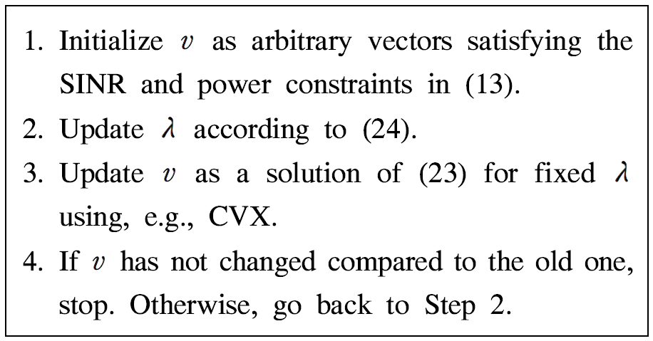
(23)[TeX:] $$\begin{array}{ll} \max _{v, \lambda} & \sum_{r=1 k}^{R_{1,1}} \sum_{\in[K]} \chi_{1,1, r}\binom{\left\|\lambda_{r, k}^S\right\|^2-}{2 \operatorname{Re}\left\{\left(\lambda_{r, k}^S\right)^H U_{1,1, r} v_k\right\}} \\ \text { s.t. } & \left|\lambda_k^C\right|^2\left(\sum_{l \in[K] \backslash\{k\}}\left|h_k^H v_l\right|^2+\sigma_C^2\right) \\ & -2 \operatorname{Re}\left\{v_k^H h_k \lambda_k^C\right\} \geq \gamma_{t h}, \forall k \in[K], \\ & \sum_{k \in[K]}\left\|v_k\right\|^2 \leq P . \end{array}$$Unlike (22), the newly formulated problem (23) involves joint optimization over the primary variables v and auxiliary variables [TeX:] $$\lambda=\left\{\lambda_{r, k}^S \in C^{N_R \times 1}\right\} \cup\left\{\lambda_k^C \in C\right\} .$$ This reformulation has two key advantages: i) For fixed v , the optimal λ that maximize the objective function and the left-hand side (LHS) of the first constraint is given in closed form as
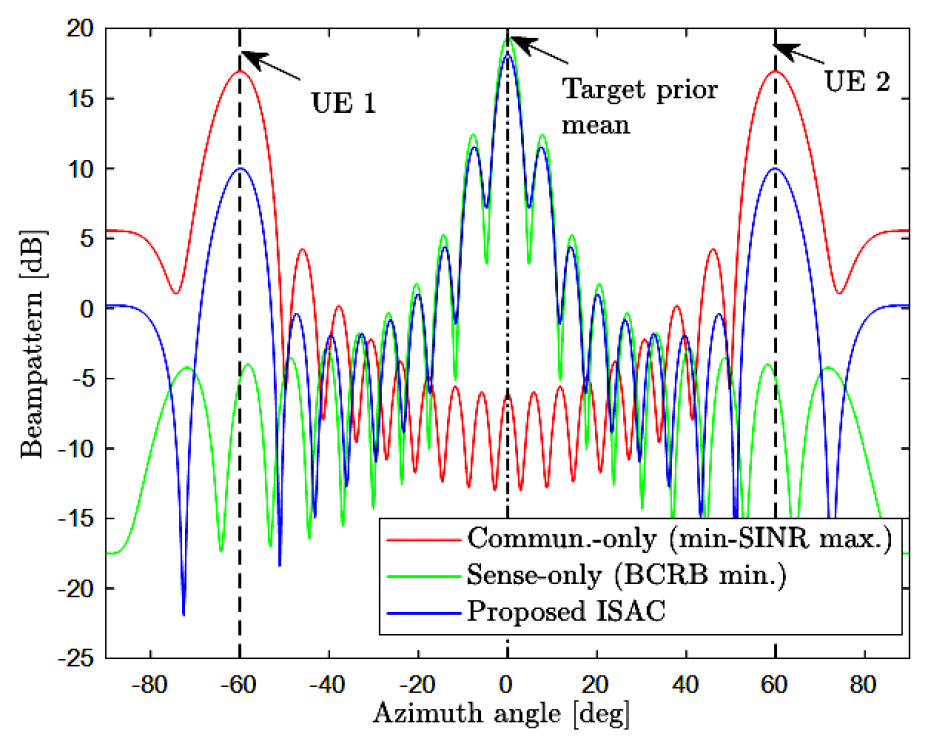
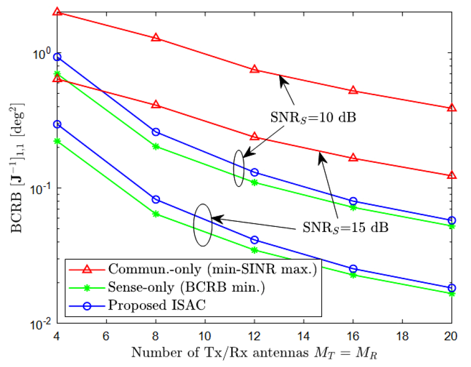
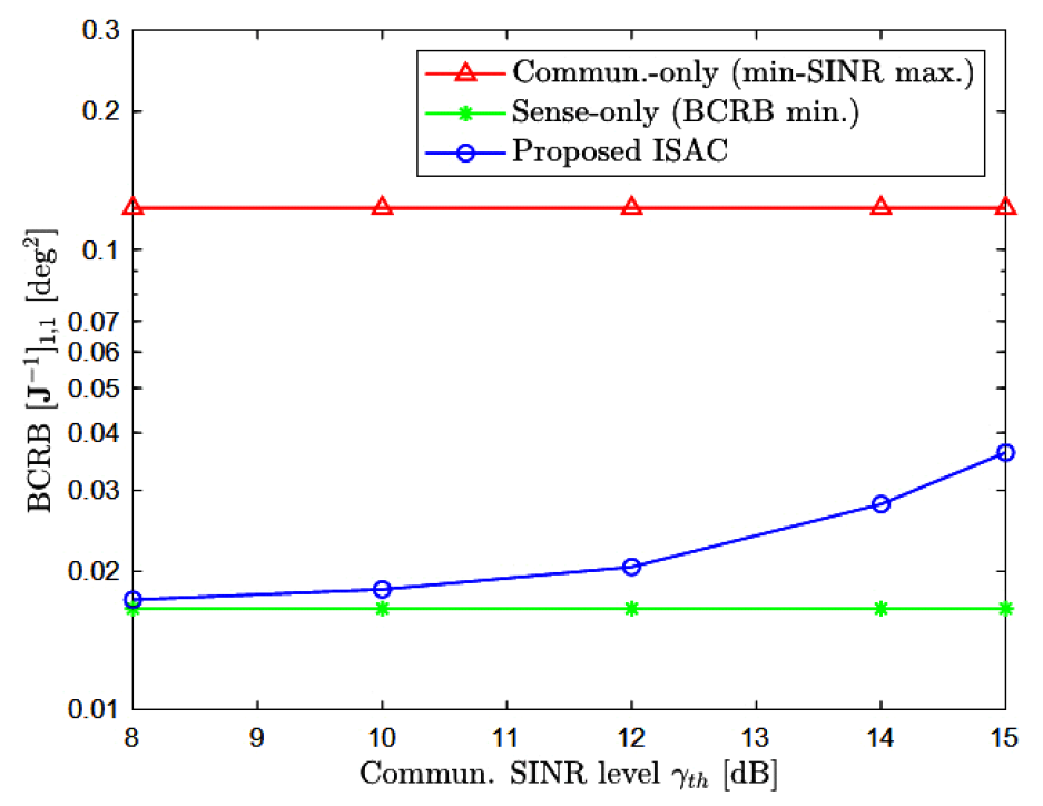
(24)[TeX:] $$\begin{aligned} & \lambda_{r, k}^S=U_{1,1, r} v_k, \\ & \lambda_k^C=\frac{h_k^H v_k}{\sum_{l \in[K] \backslash\{k\}}\left|h_k^H v_l\right|^2+\sigma_C^2} . \end{aligned}$$ii) Given fixed λ, the optimization over v becomes a convex problem, which can be efficiently solved using standard optimization solvers such as CVX[12]. Based on these insights, we adopt an alternating optimization (AO) approach, where we iteratively optimize v and λ in an alternating fashion. The detailed procedure of the proposed AO algortihm is summarized in Algorithm 1. Ⅳ. Numerical ResultsIn this section, we present numerical results to evaluate the effectiveness of the proposed ISAC beamforming design. 4.1 Simulation Setup and Baseline SchemesWe assume that the target angle θ to be setimated follows a Gaussian prior distribution [TeX:] $$\theta \sim N\left(\mu_\theta, \sigma_\theta^2\right) .$$ The channel vector [TeX:] $$h_k$$ from the BS to each C-UE k is modeled as a Rician fading channel:
where [TeX:] $$K_C$$ is the Rician K-factor, [TeX:] $$h_k^{\operatorname{LoS}}=a_T\left(\theta_k^C\right)$$ respresents the line-of-sight (LoS) component with an AoA [TeX:] $$\theta_k^C$$ relative to the BS, and [TeX:] $$h_k^{N L o S} \sim C N(0, I)$$ corresponds to the non-LoS component. Throughout the section, we set [TeX:] $$\sigma_\alpha^2=1$$ for the sensing channel. We compare the radiation beampattern and average BCRB performance of the proposed ISAC scheme against the following baseline schemes: Commun.-only: Beamforming vectors v are optimized using a max-min fairness criteriton, aiming to maximize the minimum SINR [TeX:] $$\min _{k \in[K]} \gamma_k(v)$$ while disregarding the sensing metric; Sense-only: Beamforming vectors v are optimized to minimize the BCRB [TeX:] $$\left[J^{-1}\right]_{1,1}$$ without enforcing the communication SINR constraints. Consequently, this scheme may violate the SINR requirements for C-UEs. 4.2 Numerical ResultsFig. 2 illustrates the beampatterns of the proposed ISAC scheme and baseline schemes by plotting the array response [TeX:] $$\left|a_T(\phi)\right|^2$$ versus the azimuth angle [TeX:] $$\phi$$ for a multi-user ISAC system with [TeX:] $$N_T=N_R=20,$$ T=20, [TeX:] $$S N R_C=S N R_S=20\mathrm{~dB}, \quad \gamma_{t h}=10 \mathrm{~dB},$$ K=2, [TeX:] $$K_C=\infty, \theta_1^C=-60^{\circ}, \theta_2^C=60^{\circ}, \mu_\theta=0^{\circ} \text {, } \sigma_\theta=5^\circ.$$ The sensing-only beamforming scheme concentrates most of the beam power toward the mean direction [TeX:] $$\mu_\theta=0^{\circ}$$ of the target prior distribution. Therefore, its beam power to the C-UEs is minimal, suggesting that the communication SINR constraints may not be met. In contrast, the communication-only scheme distributes the available beam power almost equally among the C-UEs’ directions [TeX:] $$\theta_1^C=-60^{\circ} \text { and } \theta_2^C=60^{\circ}$$, while the power directed toward the target prior mean is significantly lower than that of the sensing- only scheme. This suggests a substantial degradation in BCRB performance for the communication- only scheme. The proposed ISAC beamforming design achieves a well-balanced power allocation between the target prior mean direction and the AoAs of the C-UEs. Notably, in this simulated scenario, the proposed scheme achieves a BCRB performance very close to that of the sensing-only scheme while ensuring that the communication SINR constraints are satisfied. Fig. 3 presents the average BCRB as a function of the numbers of transmit/receive antennas [TeX:] $$N_T=N_R$$ in a multi-user ISAC system with T=20, [TeX:] $$S N R_C=15 \mathrm{~dB}, \gamma_{t h}=10 \mathrm{~dB}, K=2, K_C=10 \mathrm{~dB}, \theta_1^C=-60^{\circ}, \theta_2^C=60^{\circ}, \mu_\theta=0^{\circ}, \sigma_\theta=10^{\circ} .$$ As expected, the communication-only scheme exhibits the worst BCRB performance, as it does not account for the sensing metric in beamforming design. Comparing the sensing-only and proposed ISAC schemes, we observe a sensing performance loss in the ISAC scheme due to the additional constraint of satisfying communication SINR requirements. However, this loss gradually diminishes as the numbers of antenans [TeX:] $$N_T=N_R$$ increase, benefiting from enhanced beamforming capability. Fig. 4 depicts the average BCRB versus the communication SINR level [TeX:] $$\gamma_{t h}$$ for a multi-user ISAC system with [TeX:] $$N_T=N_R=20,$$ T=20, [TeX:] $$S N R_C=S N R_S=15 \mathrm{~dB}, \quad K=2, \quad K_C=10\mathrm{~dB} \theta_1^C=-60^{\circ}, \theta_2^C=60^{\circ}, \mu_\theta=0^{\circ}, \sigma_\theta=10^{\circ} .$$ When the required communication SINR [TeX:] $$\gamma_{t h}$$ is below a certain threshold, the proposed ISAC scheme achieves the same BCRB performance as the sensing-only scheme. However, as [TeX:] $$\gamma_{t h}$$ increases, the beamforming directions must shift more toward the C-UEs’ channel vectors to maintain communication quality. This adjustment reduces the beam power allocated to sensing, leading to degraded BCRB performance compared to the sensing-only scheme. Ⅴ. ConclusionWe have addressed ISAC beamforming optimization for a multi-user system, where a BS serves multiple single-antenna C-UEs while simultaneously sensing a target based on echo signals. We formulated a BCRB-based optimization problem to enhance sensing accuracy while ensuring communication reliability. Using the matrix quadratic transform, we structured the problem for efficient optimization and developed an AO algorithm that ensures monotonic convergence. Numerical results demonstrated the effectiveness of the proposed ISAC scheme in balancing sensing and communication performance as compared to sensing- or communication-oriented baseline schemes. Future work includes extending the proposed approach to a networked ISAC system, involving multiple coordinating BSs possibly with fronthaul constraints, as well as to more challenging scenarios such as simultaneous multi-target sensing or environments with interference from clutters and uplink transmissions. BiographySeok-Hwan Park2011: Ph.D. Electrical Engineering, Korea University, Seoul, Korea 2005: B.Sc. Electrical Engineering, Korea University, Seoul, Korea 2015~Current: Professor, Division of Electronic Engineering, Jeonbuk National University (JBNU), Jeonju, Korea 2024~2025:Visiting Professor, University of Toronto(UofT), Toronto, ON, Canada 2014~2015: Senior Engineer, Samsung Electronics, Suwon, Korea 2012~2014: Postdoctoral Research Associate, New Jersey Institute of Technology (NJIT), Newark, NJ, USA 2011~2012:Research Engineer, Agency for Defense Development (ADD), Daejeon, Korea [Research Interest] Wireless communications, signal processing, optimization, machine learning References
|
StatisticsCite this articleIEEE StyleS. Park, "Fractional Programming for Multi-User ISAC Beamforming Design: A Bayesian CRB Perspective," The Journal of Korean Institute of Communications and Information Sciences, vol. 50, no. 9, pp. 1397-1404, 2025. DOI: 10.7840/kics.2025.50.9.1397.
ACM Style Seok-Hwan Park. 2025. Fractional Programming for Multi-User ISAC Beamforming Design: A Bayesian CRB Perspective. The Journal of Korean Institute of Communications and Information Sciences, 50, 9, (2025), 1397-1404. DOI: 10.7840/kics.2025.50.9.1397.
KICS Style Seok-Hwan Park, "Fractional Programming for Multi-User ISAC Beamforming Design: A Bayesian CRB Perspective," The Journal of Korean Institute of Communications and Information Sciences, vol. 50, no. 9, pp. 1397-1404, 9. 2025. (https://doi.org/10.7840/kics.2025.50.9.1397)
|