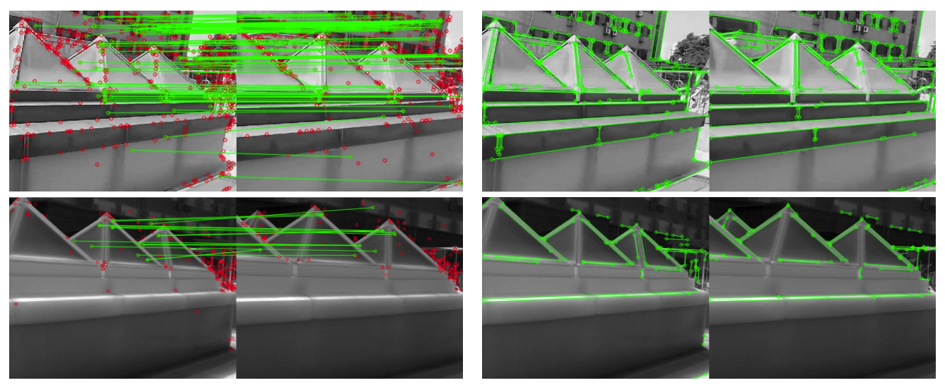
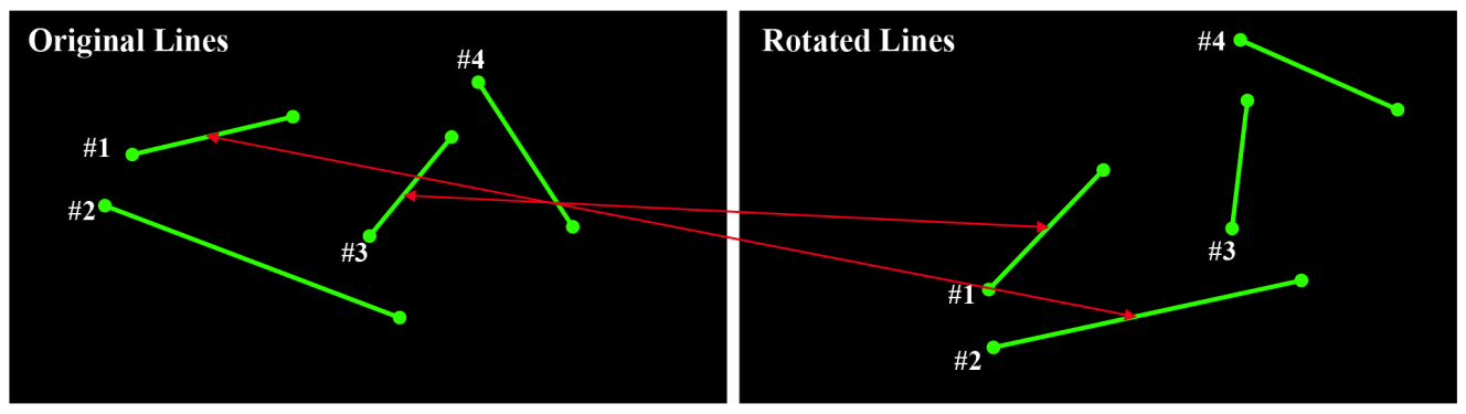
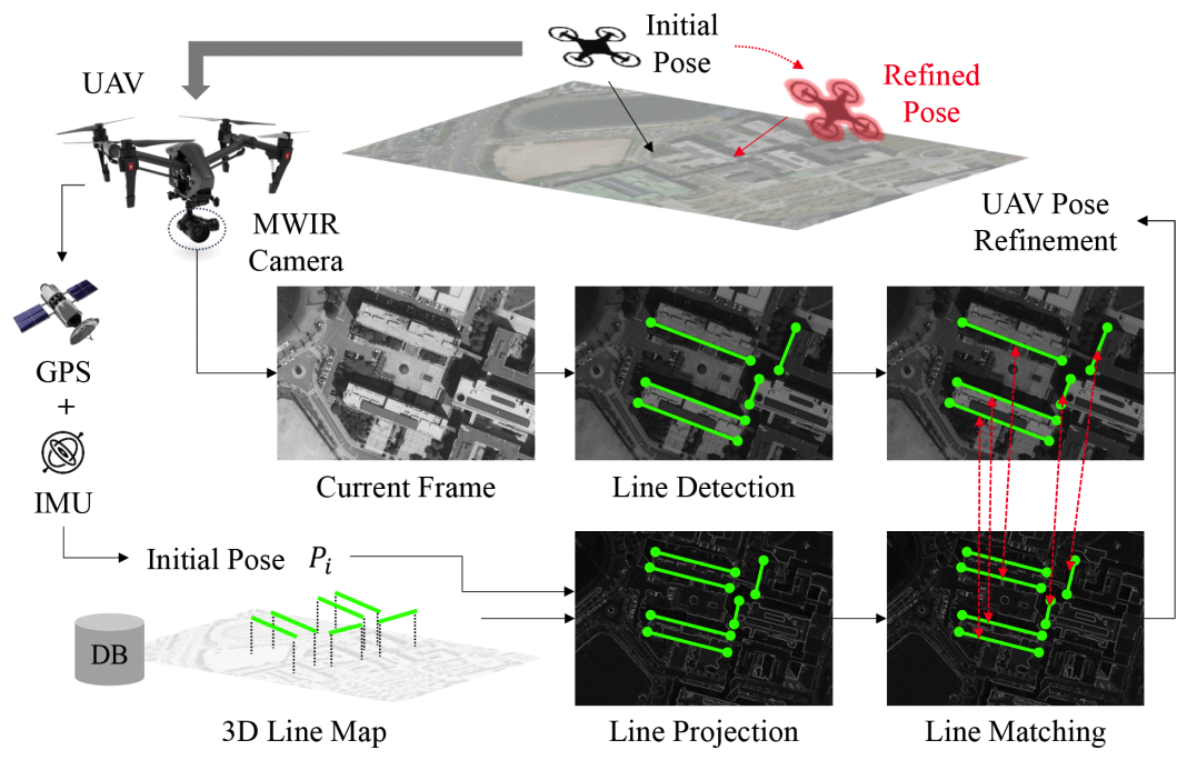
A Line-Based Unmanned Aerial Vehicle Localization Framework Using Mid-Wave Infrared Observations

Ⅰ. Introduction

The development of low-cost motors and gyroscopic sensors has led to the widespread production of unmanned aerial vehicles (UAVs), which have become essential tools for capturing aerial imagery^[1,2]. A key requirement for such tasks is accurate UAV localization, which involves estimating the vehicle’s pose by integrating various sensor inputs, including GPS data, IMU measurements, and visual features^[3]. While GPS and IMU provide initial pose estimates, visual features are commonly used to refine the UAV’s position and orientation. Many localization methods rely on visual features extracted fromvisible light (VL) imagery^[4,5]. However, VL sensors are highly sensitive to lighting conditions and have poor transmittance in adverse weather, limiting their effectiveness. To address these limitations, remote sensing imagery, particularly mid-wave infrared(MWIR), offers a promising alternative, as MWIR is less affected by lighting and weather conditions. Despite these advantages, UAV localization using MWIR imagery remains underexplored, and effective methodologies for applying localization techniques in this domain are not well established.

However, existing localization methods designed for VL images^[4,5] cannot be directly applied to UAV localization using MWIR imagery. The primary reason is that MWIR images exhibit significantly different characteristics from VL images, leading to a mismatch in the behavior of conventional visual descriptors. As shown in Fig. 1(a), keypoints extracted using the SIFT algorithm^[6] are much sparser in MWIR images due to their predominantly texture-less regions, whereas VL images yield a dense set of keypoint descriptors. In contrast, Fig. 1(b) depicts that line features detected by the EDLines algorithm^[7] show comparable results in both MWIR and VL images. This is because line detection relies primarily on strong image gradients rather than complex local descriptors, making it more robust to the modality gap between VL and MWIR

Fig. 1.

Feature detection results between (a) SIFT descriptor and (b) EDLines.

However, lines without associated descriptors are unsuitable for reliable feature matching, which is essential for UAV pose refinement. Most UAV localization methods rely on matching visual features detected in the current frame with those from previous frames. Since the UAV’s viewpoint changes over time, descriptors that are invariant to geometric transformations, such as SIFT, are commonly used to represent visual features. These descriptors allow for robust comparison of features despite changes in viewpoint or scale. In contrast, measuring the similarity between lines is inherently ambiguous without descriptive representations^[8,9]. As illustrated in Fig. 2, existing line distance metrics often result in mismatches under significant rotation or translation. Therefore, for line-based localization to be viable, a more sophisticated matching strategy must be employed.

Fig. 2.

Common mismatches between two set of lines using the angle distance of [ 9].

Motivated by these challenges, we propose a novel line-based UAV localization framework targeted for MWIR observations, which performs feature matching and pose refinement without relying on descriptors. An overview of the proposed framework is shown in Fig. 3. The UAV’s initial pose, estimated using GPS and IMU measurements, is refined using visual cues from MWIR imagery. We adopt lines as the primary visual features, as line detection proves more reliable than keypoint detection in MWIR images. Given a predefined 3D line map and the initial pose estimate, 3D lines are transformed into the UAV’s local coordinate system. These transformed lines are then matched with the detected 2D lines. Finally, the UAV pose is refined by minimizing the reprojection error between the 3D lines and their corresponding matched 2D observations.

Fig. 3.

Overview of the proposed MWIR imaging-based UAV localization method.

To address the inherent ambiguity in line matching, we design a 2D-3D line matching model capable of establishing correspondences under large rotation and translation changes. Both 2D and 3D lines are represented using Plücker coordinates^[10], which encode line geometry using direction and moment vectors rather than endpoints. This representation is significantly more stable, as endpoint-based coordinates are highly susceptible to detection noise, complicating model training. Our matching model learns the geometric structure of the 3D line map and the relationships between detected 2D lines through self-and cross-attention mechanisms^[11]. The final line correspondences are determined by solving an optimal transport problem using the matching scores predicted by the model.

Training this matching model requires a sufficiently large dataset that captures the underlying geometry of the 3D map and the relationship to its 2D projections. However, collecting labeled data for a specific 3D line map is impractical, as it requires manual annotation of 2D-3D line correspondences. To overcome this limitation, we propose a novel data augmentation strategy that generates synthetic training data in a fully automated manner. Given a 3D line map, our method samples a reference UAV pose and a randomly perturbed pose to simulate realistic viewpoint changes. It then renders 2D projections of the 3D lines from the augmented pose and adds noise to the projected lines to mimic real-world 2D line detections. By training on this synthetic dataset, our model learns to generalize effectively to real-world MWIR scenarios without requiring manually labeled ground-truth matches.

Our main contributions are summarized as follows:

· We propose a novel UAV localization framework targeted for MWIR imagery, using line-based representations for enhanced robustness under challenging sensing conditions.

· We introduce a 2D-3D line matching model that is significantly more robust to large rotational and translational variations compared to conventional matching methods

· We develop a data augmentation strategy that automatically generates realistic synthetic training data, enabling effective model training without the need for manually annotated real-world data.

Ⅱ. Methodology

2.1 Notations

Let [TeX:] $$\mathscr{L}_{3 D}=\left\{L_i \mid L_i \in \mathbb{R}^{3 \times 2}, i=1, \ldots, M\right\}$$ denote the set of predefined 3D lines, where each line Li is represented by its two endpoints in world coordinates, typically corresponding to geological landmarks. Similarly, let [TeX:] $$\mathscr{L}_{2 D}=\left\{l_i \mid l_i \in \mathbb{R}^{2 \times 2}, i=1, \ldots, N\right\}$$ denote the set of 2D lines detected fromthe current MWIR image. The UAV’s initial pose, estimated from sensor data, is denoted by [TeX:] $$P_i=\left[R_i / t_i\right]$$], where [TeX:] $$R_i \in \mathrm{SO}(3)$$ is the 3D rotation matrix and [TeX:] $$t_i \in \mathbb{R}^{3 \times 1}$$ is the translation vector. The refined pose, obtained after line matching and pose optimization, is denoted by [TeX:] $$P_r=\left[R_r / t_r\right]$$, with analogous definitions for R_r and t_r. The transformed 3D line map [TeX:] $$\tilde{\mathscr{L}}_{3 D}$$, expressed in the UAV coordinate system defined by P_i, is given by:

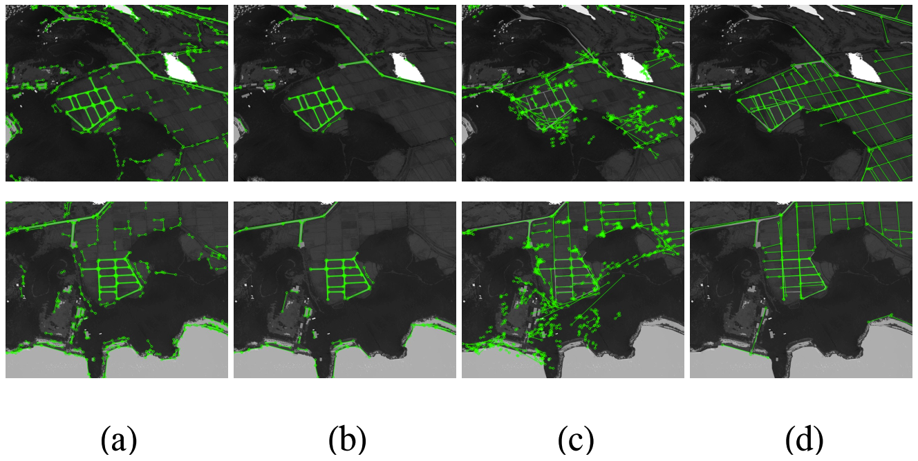
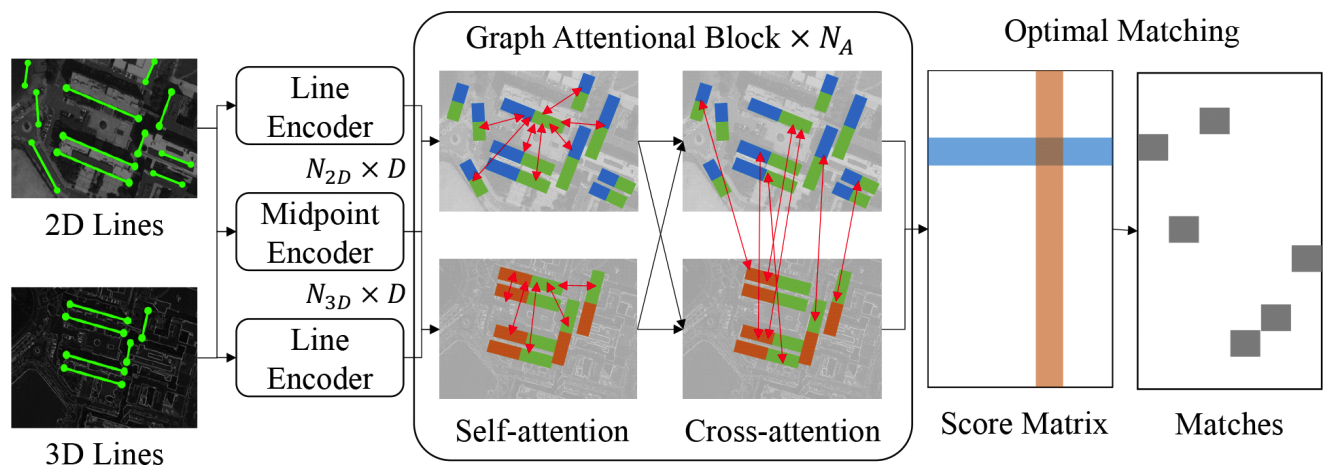
2.2 Line Detection

As various line detection methods exist, it is important to select the approach most suitable for MWIR-based UAV localization. Broadly, line detection methods can be categorized into two groups: (1) image processing-based methods and (2) learning-based methods. We compare two widely used methods from each category: LSD^[12 and EDLines^[7 for image processing-based approaches, and AFM^[13 and MLSD^[14 for learning-based approaches. The comparison results are shown in Fig. 4.

Fig. 4.

Lines detected in MWIR images using (a) LSD, (b) EDLines, (c) AFM, and (d) M-LSD.

As illustrated in Fig. 4(a) and Fig. 4(b), image processing-based methods such as LSD and ED-Lines reliably detect prominent lines in MWIR images by leveraging strong image gradients. In contrast, as shown in Fig. 4(c) and Fig. 4(d), learning-based methods such as AFM and M-LSD perform poorly in this domain, exhibiting significant noise and failing to extract meaningful lines. This degradation stems from the fact that these models are trained on VL images and thus learn feature distributions specific to the VL domain. Adapting them to MWIR imagery would require substantial retraining with annotated MWIR data, which is expensive and difficult to obtain. Given these observations, we conclude that image processing-based line detection methods are more suitable for MWIR-based UAV localization, as they require no training and are robust to domain shifts. Among them, we adopt EDLines over LSD, as it produces fewer but more salient lines, reducing clutter and improving subsequent line matching performance.

2.3 Line Matching

As previously shown in Fig. 2, conventional distance-based line matching methods^[8,9] often result in mismatches, as the distance between two lines is inherently ambiguous without known correspondences. However, meaningful matches can still be inferred by leveraging the geometric relationships among neighboring lines. To exploit this relational information, we design a 2D-3D line matching model inspired by the graph attentional architecture^[11], as illustrated in Fig. 5. Our model begins by encoding the detected 2D lines Lﾘ2D and the transformed 3D lines Lﾘ3D using a line encoder and a midpoint encoder. To match the dimensionality between 2D and 3D lines, we represent the 2D lines in homogeneous coordinates. We then represent each line using Plücker coordinates^[10], which is composed of direction and moment vectors. Given a 3D [TeX:] $$\tilde{L}_i=\left[\tilde{x}_{1, i}, \tilde{x}_{2, i}\right]$$ where [TeX:] $$\tilde{x}_{1, i}$$ and [TeX:] $$\tilde{x}_{2, i}$$ are its endpoints, the Plücker coordinates of [TeX:] $$\tilde{L}_i$$ is computed as:

Fig. 5.

Architecture of the proposed 2D-3D line matching model.

where d is the direction vector and m is the moment vector. The moment vector is the normal of the plane formed by the two endpoints and the origin.

For 2D lines, the direction vector is constrained by the image plane, and the moment vector m uniquely defines the line up to scale. Thus, we normalize the moment vector to obtain the final representation [TeX:] $$\bar{m}=m\|m\|$$. Each 2D or 3D line is then encoded into a D-dimensional feature vector using a multi-layer perceptron (MLP), referred to as the line encoder. To differ-entiate between colinear lines, which cannot be distinguished solely by the moment vector, we also encode the midpoint [TeX:] $$\tilde{x}_{m, i}=\left(\tilde{x}_{1, i}+\tilde{x}_{2, i}\right) / 2$$ of each line using a separate MLP, referred to as the midpoint encoder. The outputs of the line encoder and midpoint encoder are summed to produce the final line feature [TeX:] $$f_i \in \mathbb{R}^D$$, which is then passed to the graph attentional module.

The graph attentional module and matching mechanism follow the formulation of^[11]. Given the encoded 2D and 3D line features [TeX:] $$F^{2 D}=\left[f_1^{2 D}, \ldots, f_{N_{2 D}}^{2 D}\right]$$ and [TeX:] $$F^{3 D}=\left[f_1^{3 D}, \ldots, f_{N_{3 D}}^{3 D}\right]$$, the module computes both self-attention (within each set) and cross-attention(between sets), allowing contextual interactions among and across line features. This attentional block is repeated N_A times to progressively refine the features. To obtain the final matching, we first compute a score matrix which quantifies the similarity between refined 2D and 3D line features. The score matrix [TeX:] $$S \in \mathbb{R}^{\left(N_{3 D}+1\right) \times\left(N_{2 D}+1\right)}$$ is computed using the inner-product between the refined features at the final layer L, augmented with a learnable dustbin score z for unmatched lines:

where [TeX:] $$\mathscr{I}_{3 D}=\left\{1,2, \ldots N_{3 D}\right\}$$ and [TeX:] $$\mathscr{I}_{2 D}=\left\{1,2, \ldots N_{2 D}\right\}$$. To obtain the assignment, we solve an optimal transport problem over S using the Sinkhorn algorithm^[15]], which provides a differentiable approximation of the Hungarian algorithm^[16]. This results in a soft assignment matrix [TeX:] $$\tilde{A}$$, which represents the model’s confidence in each 2D-3D line pair.

The entire network is trained end-to-end using a loss function that supervises both matched and unmatched primitives:

where [TeX:] $$\hat{\mathscr{M}}$$ denotes the set of ground-truth 2D-3D line correspondences, and [TeX:] $$\hat{\mathscr{M}}_i$$, [TeX:] $$\hat{\mathscr{M}}_j$$ represent the sets of matched indices in 2D and 3D lines, respectively. The first term maximizes the confidence of correct matches, while the remaining terms guide the model to assign unmatched lines to the dustbin entry. Finally, the set of predicted matches is obtained by selecting, for each 3D line, the 2D line with the highest assignment score:

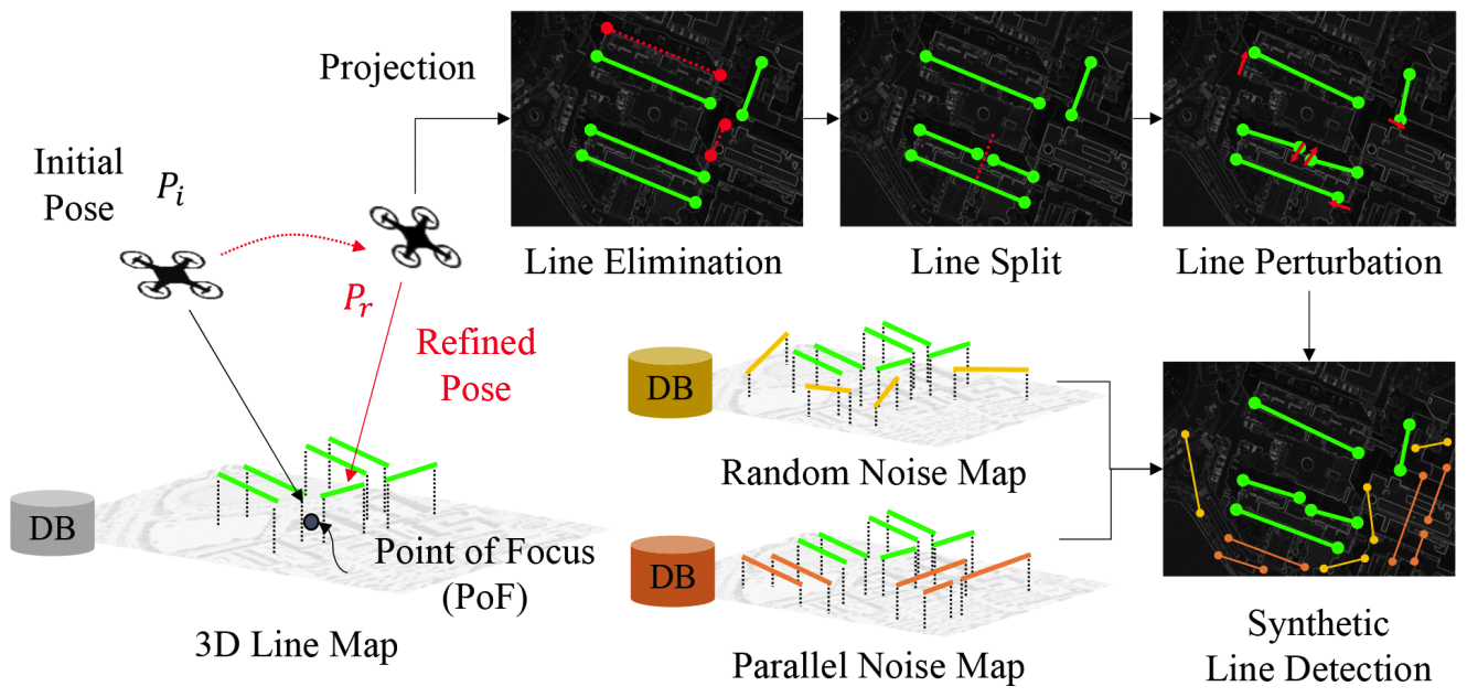
2.4 Synthetic Data Augmentation

While careful model design is important, its effectiveness ultimately depends on the availability of appropriate training data. This is particularly critical for our 2D-3D line matching model, which must learn the geometric relationships specific to a given 3D line map. However, collecting such training data is laborintensive, requiring MWIR image sequences, 2D line detection, and manual annotation of correspondences between 2D and 3D lines. To address this challenge, we propose a novel synthetic data augmentation method that generates realistic 2D-3D line pairs with minimal domain discrepancy, enabling effective model training without manual labeling. The overall augmentation process is shown in Fig. 6.

Fig. 6.

Line matching data augmentation process.

First, a point-of-focus (PoF) xPoF is sampled near the 3D line map [TeX:] $$\mathscr{L}_{3 D}$$. This is achieved by drawing a 3D point from a Gaussian distribution defined by the mean and standard deviation of the midpoints of the lines in [TeX:] $$\mathscr{L}_{3 D}$$. Next, we sample a random distance [TeX:] $$r \in[n, f]$$, azimuth angle [TeX:] $$\theta \in[0,2 \pi]$$, elevation angle [TeX:] $$\phi \in[0, \pi / 2]$$, and twist angle [TeX:] $$\psi \in[-\pi / 3, \pi / 3]$$, where n and f denote the near and far bounds of the sampling radius. The initial UAV pose Pi is then defined as:

where [TeX:] $$R_x(\cdot)$$, [TeX:] $$R_y(\cdot)$$, [TeX:] $$R_z(\cdot)$$ are rotation matrices around the respective axes, and [TeX:] $$\hat{e}_x$$ is the unit vector alongthe x-axis. We can now obtain the transformed 3D line map [TeX:] $$\mathscr{L}_{3 D}$$ given the initial UAV pose using Eq.(1). The next step is to generate synthetic 2D lines to make pairs with the transformed 3D lines. We first transform the initial pose to a new pose P_r, which will be the target refined pose. The refined pose is derived by adding random rotation and translation as follows:

where [TeX:] $$\delta \psi, \delta \phi, \delta \theta, \delta r_x, \delta r_y, \delta r_z, \hat{e}_y, \hat{e}_z$$, are random rotation angles and random translation distances with respect to x, y, z axes, and unit vectors in the y, z-axis direction, respectively.

Given the refined pose P_r, we project the 3D line map [TeX:] $$\mathscr{L}_{3 D}$$ to the Pr to obtain the projected 2D line map [TeX:] $$\mathscr{L}_{2 D}^{\prime}=\left\{l_i^{\prime} \mid l_i^{\prime} \in \mathbb{R}^{2 \times 2}, i=1, \ldots, N_{3 D}\right\}$$. Each line in [TeX:] $$L_i=\left[x_{1, i}, x_{2, i}\right] \in \mathscr{L}_{3 D}$$ is projected by transforming its endpoints and applying the pinhole camera model:

where K is the camera intrinsics and [TeX:] $$\pi(\cdot)$$ denotes the perspective projection function:

From the projected 2D line map [TeX:] $$\mathscr{L}_{2 D}^{\prime}$$, we apply line noises which are frequently observed in real 2D linedetection as in Fig. 4. For each 2D line [TeX:] $$l_{2 D}^{\prime} \in \mathscr{L}_{2 D}^{\prime}$$ we randomly eliminate, split and perturb their endpoints.

After the target lines are augmented, additional noise lines are introduced to simulate realistic detection artifacts. Specifically, lines are sampled from two sources: a random noise map [TeX:] $$\mathscr{L}_R$$ and a parallel noise map [TeX:] $$\mathscr{L}_P$$. The random noise map contains lines generated near the 3D line map [TeX:] $$\mathscr{L}_{3 D}$$, while the parallel noise map includes lines that are spatially aligned and oriented parallel to lines in [TeX:] $$\mathscr{L}_{3 D}$$. Using the same projection process applied to [TeX:] $$\tilde{\mathscr{L}}_{3 D}$$, both [TeX:] $$\mathscr{L}_R$$ and [TeX:] $$\mathscr{L}_P$$ are projected to the refined pose P_r using Eq.(8), producing the projected sets [TeX:] $$\mathscr{L}_R^{\prime}$$ and [TeX:] $$\mathscr{L}_P^{\prime}$$. These are then added to the augmented target lines [TeX:] $$\mathscr{L}_2D^{\prime}$$ to generate the final synthetic 2D line detection set [TeX:] $$\tilde{\mathscr{L}}_{2 D}$$:

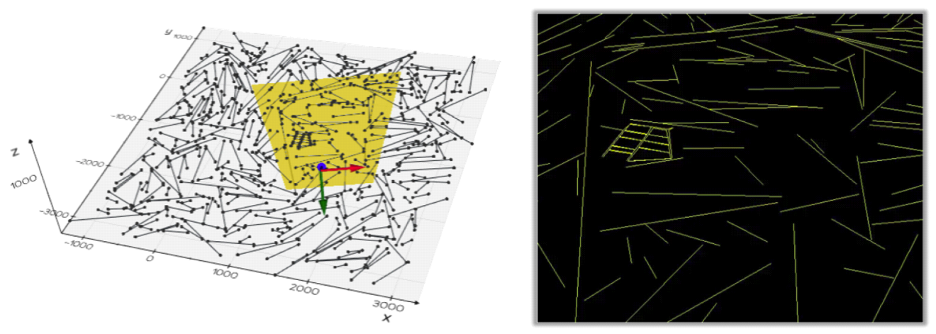
Since both the [TeX:] $$\tilde{\mathscr{L}}_{3 D}$$ and [TeX:] $$\tilde{\mathscr{L}}_{2 D}$$ are generated from the same underlying [TeX:] $$\mathscr{L}_{3 D}$$, the ground-truth correspondences can be automatically derived without the need for manual labeling. An example generated syntheticline is shown in Fig. 7.

Fig. 7.

Example visualization of the synthetic line detection generation process.

2.5 Pose Refinement

Finally, given the predicted matches [TeX:] $$\mathscr{M}$$ between the detected 2D lines [TeX:] $$\tilde{\mathscr{L}}_{2 D}$$ and transformed 3D lines [TeX:] $$\tilde{\mathscr{L}}_{3 D}$$, we can now estimate the refined pose P_r of the UAV from the initial pose P_i. Since the transformed lines [TeX:] $$\tilde{\mathscr{L}}_{3 D}$$ originate from the 3D line map [TeX:] $$\mathscr{L}_{3 D}$$, their identities are preserved, allowing us to directly associate [TeX:] $$\tilde{\mathscr{L}}_{2 D}$$ with the corresponding lines in [TeX:] $$\mathscr{L}_{3 D}$$. The refined pose P_r is obtained by minimizing the following energy function:

where [TeX:] $$l_i^{\prime}$$ and [TeX:] $$m_i^{\prime}$$ represent the direction and moment vectors of the detected 2D line i, and [TeX:] $$\tilde{l}_j$$ and [TeX:] $$\tilde{m}_j$$ are the corresponding direction and moment vectors of the projected 3D line j. The scalar w is a weighting factor that controls the relative contribution of the moment term. It is evident from Eq.(8) that [TeX:] $$l_i^{\prime}$$ is a function of the refined pose P_r. Given the endpoints of [TeX:] $$l_i^{\prime}$$, the corresponding moment vector [TeX:] $$m_i^{\prime}$$ can be computed using Eq.(2). Since [TeX:] $$l_i^{\prime}$$ and [TeX:] $$m_i^{\prime}$$ are differentiable with respect to P_r, the energy function E(P_r) can be efficiently minimized using gradient-based non-linear optimization methods.

2.6 Implementation Details

For the 2D-3D line matching model, we use a feature dimension of D = 128 and apply a total of N_A= 3 graph attention blocks. To generate the synthetic training dataset, we sample 10,000 distinct pairs of initial and refined UAV poses (P_i, P_r) following the formulations in Eq.(6) and Eq.(7). The random distance r used to determine the initial pose is sampled uniformly from the range [n, f] with bounds n =10 and f = 200. Azimuth θ, elevation ϕ, and twist ψ angles are also sampled uniformly within their respective domains. For generating the refined pose P_r, random rotational perturbations δψ, δϕ, δθ are sampled from the range [−π/12, π/12], and translational perturbations δr_x, δr_y, δr z are sampled from [−10, 10]. To simulate realistic noise in 2D line detection, we generate 400 random and parallel lines around the 3D line map, ensuring no intersection with the existing lines. The 2D-3D line matching model is trained for 200 epochs using the Adam optimizer^[17], with a learning rate of 5×10^-4 and a batch size of 64. For pose refinement, the weighting factor in the energy function is set to w = 10⁻⁵, and the optimization is performed using the Levenberg-Marquardt algorithm^[18].

Ⅲ. Experiments

3.1 Dataset

Fig. 8.

Our simulated UAV flight dataset: (a) simulated flight sequences, (b) annotated 3D line map. Rendered images of Dive (Top) and Around (Bottom) sequences in (c) MIWR, (d) VL, (e) night time VL, (f) foggy VL.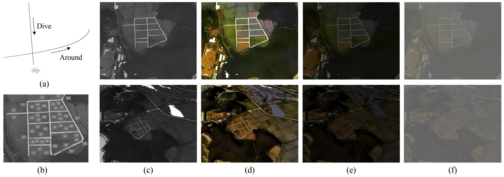

To evaluate the effectiveness of our MWIR-based UAV localization framework, we constructed a simulated UAV flight dataset using the physics-based sensor simulator provided by OKTAL-SE^[19], which is widely adopted for generating realistic optical imagery^[20,21]. The simulation was performed over a detailed 3D model of Sinjin Island, with rendered images generated in both MWIR and VL bandwidth. We defined two distinct UAV flight patterns, Around and Dive, as illustrated in Fig. 8(a). These patterns are inspired by widely adopted flight configurations in benchmarks such as the EuRoC MAV Dataset^[22], which provide both easy and hard trajectories to evaluate robustness. In our dataset, the Dive sequence represents a relatively straightforward trajectory with limited viewpoint variation, whereas the Around sequence introduces significant angular and positional diversity, simulating more challenging conditions for localization.

The sensors used in both simulations have a resolution of 640×512 pixels. The intrinsic parameters are set to f_x = f_y = 1140, with a principal point at (p_x, p_y) = (320, 256), while assuming negligible camera distortion. Each sequence lasts 15 seconds and is rendered at 30 frames per second, resulting in a total of 450 frames per sequence. All flight paths were simulated around the annotated 3D line map of Sinjin Island, which consists of geologically meaningful structural lines as shown in Fig. 8(b). To simulate realistic flight conditions, we added random rotational and translational perturbations to the smooth UAV trajectories, following the formulation in Eq.(7). During each simulation, both the UAV pose and the corresponding images were recorded for ground-truth reference. Importantly, our 2D-3D line matching model is trained exclusively on synthetic data generated from the 3D line map of Sinjin Island, without using any annotated MWIR or VL image sequences. Sample MWIR and VL renderings from the Dive and Around sequences are shown in Fig. 8(c) and (d), respectively.

To further validate the advantages of MWIR imagery over visible light (VL) under adverse conditions, we additionally rendered VL versions of both the Dive and Around sequences under two challenging scenarios. The first scenario simulates night-time conditions, where low-light settings were applied toreduce overall image brightness and contrast, as shown in Fig.8(e). The second scenario depicts foggy weather, in which visibility was degraded by overlaying a semitransparent gray veil across the images, as illustrated in Fig.8(f). These conditions are designed to reflect realworld challenges where VL-based localization methods often fail, thereby emphasizing the robustness of MWIR-based localization.

3.2 Evaluation Metrics

To assess the performance of our MWIR-based UAV localization framework, we adopt standard evaluation metrics that are widely used in the visual localization and SLAM literature. Specifically, we evaluate translation and rotation error following established protocols in [4-5], and 2D-3D line matching precision, as commonly used in the feature matching literature^[11]. The translation error E_t> measures the accuracy of the estimated UAV position relative to the ground-truth trajectory. Given the predicted translation [TeX:] $$\hat{t}_i i$$ and ground-truth translation t_i at frame i, the error is defined as:

where N is the total number of frames, and [TeX:] $$\|\cdot\|$$ denotes the Euclidean norm. The rotation error ER quantifies the angular deviation between the estimated rotation matrix [TeX:] $$\hat{R}_i$$ and the ground-truth rotation matrix R_i, and is computed as:

where Tr(·) denotes the matrix trace. This yields the mean angular error in degrees across all frames. Finally, precision is used to evaluate the accuracy of the predicted 2D-3D line correspondences. A predicted match is considered a true positive (TP) if it correctly matches the ground-truth line pair, and a false positive (FP) otherwise. The precision is then defined as:

which reflects the proportion of correct matches among all predicted matches.

3.3 Quantitative Evaluation

3.3.1 Effect of Visual Refinement

We first compared our method against baseline sensor configurations: raw GPS, raw IMU, GPS+IMUfusion, and our full pipeline, GPS+IMUwith visual refinement. GPS is modeled as ground-truth positionscorrupted with zero-mean Gaussian noise to approximate consumer-grade accuracy (20mmean position)[23]. Note that raw GPS provides position only.

The IMU baseline synthesizes gyro/accel signals with white noise and bias random walks and recovers state via strapdown mechanization^[24]. The GPS+IMU base-line uses a loosely coupled EKF with position-only updates^[25], while our method further refines the fused pose via 2D-3D line correspondences. As shown in Table 1, GPS is noisy and provides no orientation, while IMU alone drifts and yields large translation errors. The GPS+IMU fusion approach reduces these errors but remains noise-limited. With using visual refinement, our method achieves the lowest translation and rotation errors, demonstrating the effectiveness of the proposed framework.

3.3.2 Comparison with VL-based Methods

We evaluated our method on both the Around and Dive sequences by measuring trajectory estimation accuracy and 2D-3D line matching precision. To assess the effectiveness of our MWIR-based localization framework, we compared it against two recent state-of-the-art methods developed for VL imagery, ORB-SLAM3^[4] and DPVO^[5], on both VL and MWIR image sequences. ORB-SLAM3 is a classical simultaneous localization and mapping (SLAM) system that relies on handcrafted feature descriptors for keypoint detection and matching. DPVO is a deep learning-based visual odometry method that estimates camera motion by learning to match local image patches across frames for consistent frame-to-frame tracking. The trajectories for both ORB-SLAM3 and DPVO were estimated directly from the simulated image sequences. Since the estimated trajectories may differ from the groundtruth in scale, orientation, and translation, we aligned them using the Umeyama similarity transformation^[26] to enable fair comparison. As both ORB-SLAM3 and DPVO do not perform 2D-3D line matching, we report only pose estimation results for these methods. The full comparison is summarized in Table 2.

As summarized in Table 2, the VL-based baselines behave as expected: they are reasonable on clean VL (e.g., ORB-SLAM3: E_t = 12.2 m, DPVO: Et = 10.1 m) but degrade severely under VL-Night/Foggy (e.g., ORB-SLAM3 total Et ≈ 99-137 m; DPVO Et ≈ 92-119 m). When run on MWIR, both also deteriorate (ORB-SLAM3: 70.8 m, 15.1°; DPVO: 52.1 m, 11.3°), reflecting sparse keypoint detections in MWIR and modality issues due to VL-trained patch trackers. In contrast, our method maintains low error across modalities, 4.7 m/2.4° on VL and 4.9 m/2.5° on MWIR, and degrades more gracefully in VL-Night/Foggy (7.7-9.1 m, 3.5°-4.1°). These gains come from robust 2D-3D line matching, which is less sensitive to illumination and texture; the model achieves approximately 0.82 (82%) precision on MWIR overall (0.87onAround), enabling accurate pose refinement.

3.4 Qualitative Evaluation

3.4.1 Trajectory Visualization

We visualize the trajectories estimated by baseline sensor configurations and our framework in Fig.9(a) and (b). As expected, IMU-only suffers pronounced drift while GPS is reasonably accurate in positionbut does not provide orientation information. However, the loosely coupled GPS+IMU baseline still drifts as inertial errors accumulate, highlighting the limitation of localization in the absence of visual refinement. We also visualize the estimated trajectories also VL-based methods in Fig. 9(c) and (d). In Fig. 9(c), the Dive sequence involves less camera rotation than Around, resulting in relatively better performance for both ORB-SLAM3 and DPVO. As shown in Fig. 9(d), during the Around sequence, both ORB-SLAM3 and DPVO deviate significantly from the ground-truth trajectory from the beginning of the sequence. This degradation is primarily caused by the modality gap between VL and MWIR imagery, which leads to unreliable descriptor and patch matching. However, the estimated trajectories still exhibit instability, again due to poor descriptor and patch matching in the MWIR domain. In contrast, our method produces a more accurate and stable trajectory in both sequences, demonstrating its robustness and reliability under MWIR imaging conditions

Fig. 9.

Qualitative visualizations of trajectories. Comparison with baseline sensor configurations on (a) Dive and (b) Around sequences. Comparison between conventional methods using MWIR input on (a) Dive sequence (b) Around sequences.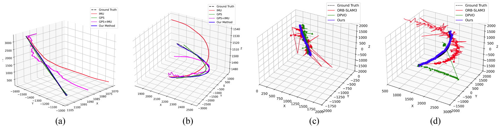

3.4.2 Matching and Refinement Visualization

We also visualize the 2D-3D line matching results between the transformed [TeX:] $$\tilde{\mathscr{L}}_{3 D}$$ line map and the detected [TeX:] $$\tilde{\mathscr{L}}_{2 D}$$ lines . Fig. 10(a) presents qualitative results for both the Around and Dive sequences. In both cases, our matching model successfully establishes correct correspondences, even under substantial viewpoint changes involving significant rotation and translation. Additionally, as shown in the rightmost matching visualization, the model remains robust to various line detection noises such as line elimination, splitting, and endpoint perturbation, which frequently occur when the UAV approaches the target lines. Despite these challenges, our model consistently identifies correct matches, demonstrating strong robustness to real-world detection artifacts. To further assess the effectiveness of pose refinement, we visualize the projections of [TeX:] $$\tilde{\mathscr{L}}_{3 D}$$ before and after refinement in Fig. 10(b). In these visualizations, the red lines represent the projected 3D lines, while the green lines indicatethe matched 2D detections. As shown in the second row of Fig. 10(b), the alignment between projected and detected lines significantly improves after pose refinement, confirming the accuracy of the estimated pose.

Fig. 10.

Qualitative visualizations of (a) 2D-3D line matching and (b) reprojection of 3D lines after pose refinement.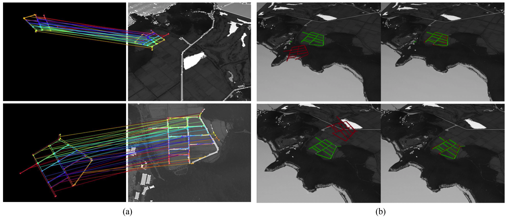

3.5 Ablation Studies

We performed ablation studies to investigate the impact of both the synthetic data augmentation strategy and key parameters of the 2D-3D line matching model. To evaluate the effectiveness of the augmentation strategy, we compared 2D-3D line matching accuracy under four settings: no augmentation, target line augmentation only, random line augmentation only, and both augmentations combined. The results, summarized in Table 3, show that without random line augmentation, the model achieves only 4-7% precision, whereas adding random line augmentation increases precision significantly, reaching up to 70%. Although target line augmentation alone does not significantly improve performance, it effectively reduces false positives. When combined with random augmentation, it improves precision by up to 11.35%, which is particularly beneficial as reducing false matches directly contributes to more accurate pose refinement.

We also searched for the optimal parameter settings of our matching model by varying the feature dimension size D and the number of attention blocks N_A. As shown in Table 4, the model achieved the highest matching precision when the feature dimension was set to D = 128. A lower feature dimension resulted in insufficient model capacity, while higher dimensions led to overfitting and degraded performance. Similarly, the best results for the number of attention blocks were observed at N_A = 3. Increasing the number of attention blocks beyond this did not yield further improvements and instead introduced more false positives, which negatively affects pose refinement.

3.6 Runtime Evaluation

As efficient onboard processing is crucial for realtime UAV localization, we evaluate the computational performance of our proposed framework across two hardware platforms: a standard PC and an embedded system. The evaluation setup is shown in Fig. 11(a) The PC is equipped with an Intel Core i7-6700 CPU and an NVIDIA GeForce GTX 1050 Ti GPU. The embedded platform, shown in Fig. 11(b), is an NXPi.MX 8M Plus^[27], a low-power board suitable for UAV deployment. The software pipeline of our framework is illustrated in Fig. 11(c), where multiprocessing is employed to parallelize the key modules.

Fig. 11.

Runtime analysis hardware and software settings. (a) Evaluation setup (b) NXP i.MX 8M Plus board (c) Software pipeline with multiprocessing.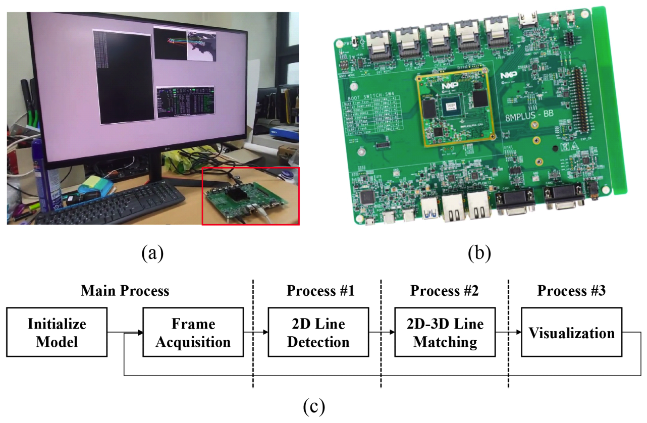

The overall runtime evaluation is conducted as follows. The 2D-3D line matching model is first initialized in the main process and converted to ONNX^[28] format for lightweight and fast inference. The pipeline begins in the main process, simulating frame acquisition by reading MWIR image sequence frame-byframe saved in a local directory. Three subprocesses are then spawned to handle the core tasks: Process #1 performs 2D line detection from the current MWIR frame, Process #2 conducts 2D-3D line matching using the ONNX model, and Process #3 performs pose refinement and visualization. The acquired frames are passed to Process #1, which performs 2D line detection. The detected lines are then sequentially forwarded to Process #2 for 2D-3D line matching, and subsequently to Process #3 for pose refinement and visualization, completing the full localization loop. Table 5 summarizes the runtime of each module and the overall throughput. The framework runs at average 61 FPS on the standard PC and 20.3 FPS on the embedded board, confirming its real-time capability even on resource-constrained hardware.

Ⅳ. Conclusion

We proposed a novel UAV localization framework for MWIR imagery, addressing the limitations of VL-based methods under challenging visibility conditions. Our approach leverages 2D-3D line matching between MWIR-detected lines and a predefined 3D line map, enabled by a robust matching model trained entirely on a synthetically augmented dataset. The framework achieves high matching precision and accurate pose refinement, demonstrating strong performance compared to VL-based baselines on simulated MWIR flights. It also runs in real-time on both desktop and embedded platforms, supporting practical deployment. A current limitation is the reliance on a predefined 3D line map. In future work, we aim to extend our framework to handle unseen environments by generalizing the matching model for online or map-free localization.